Chapter 12 Forecasting Operations Management 6 th Edition

Chapter 12 Forecasting Operations Management - 6 th Edition Roberta Russell & Bernard W. Taylor, III Copyright 2009 John Wiley & Sons, Inc. Beni Asllani University of Tennessee at Chattanooga

Lecture Outline : เพอใหนกศกษาเขาใจหวขอตอไปน w Strategic Role of Forecasting in Supply Chain Management w Components of Forecasting Demand w Time Series Methods w Forecast Accuracy w Time Series Forecasting Using Excel w Regression Methods Copyright 2009 John Wiley & Sons, Inc. 2

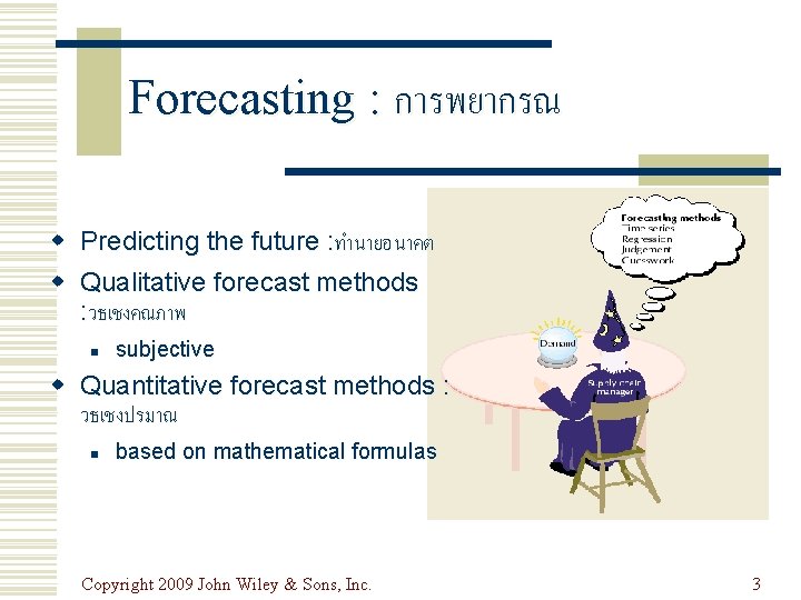
Forecasting : การพยากรณ w Predicting the future : ทำนายอนาคต w Qualitative forecast methods : วธเชงคณภาพ n subjective w Quantitative forecast methods : วธเชงปรมาณ n based on mathematical formulas Copyright 2009 John Wiley & Sons, Inc. 3

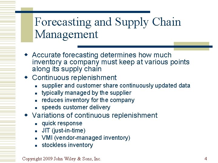
Forecasting and Supply Chain Management w Accurate forecasting determines how much inventory a company must keep at various points along its supply chain w Continuous replenishment n n supplier and customer share continuously updated data typically managed by the supplier reduces inventory for the company speeds customer delivery w Variations of continuous replenishment n n quick response JIT (just-in-time) VMI (vendor-managed inventory) stockless inventory Copyright 2009 John Wiley & Sons, Inc. 4

Forecasting w Quality Management n Accurately forecasting customer demand is a key to providing good quality service w Strategic Planning n Successful strategic planning requires accurate forecasts of future products and markets Copyright 2009 John Wiley & Sons, Inc. 5

Time Frame : ระยะเวลา w Indicates how far into the future is forecast n Short- to mid-range forecast : ระยะสน กบระยะกลาง typically encompasses the immediate future l daily up to two years : ประจำวน จนถง 2 ป l n Long-range forecast : ระยะยาว l usually encompasses a period of time longer than two years : มากกวา 2 ป Copyright 2009 John Wiley & Sons, Inc. 7

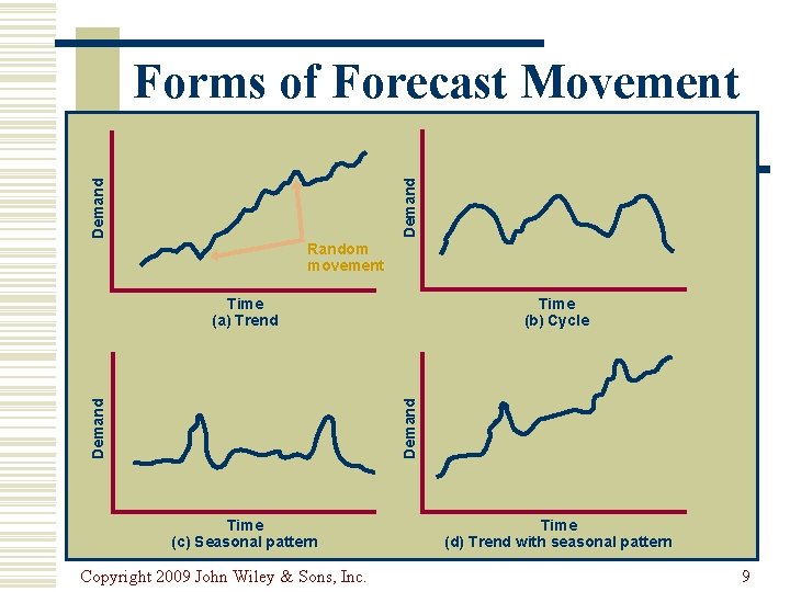
Demand Behavior : พฤตกรรมของความตองการ w Trend : แนวโนม n a gradual, long-term up or down movement of demand w Random variations : ความแปรปรวนโดยสม n movements in demand that do not follow a pattern w Cycle : วฏจกร n an up-and-down repetitive movement in demand w Seasonal pattern : ฤดกาล n an up-and-down repetitive movement in demand occurring periodically Copyright 2009 John Wiley & Sons, Inc. 8

Demand Forms of Forecast Movement Random movement Time (b) Cycle Demand Time (a) Trend Time (c) Seasonal pattern Copyright 2009 John Wiley & Sons, Inc. Time (d) Trend with seasonal pattern 9

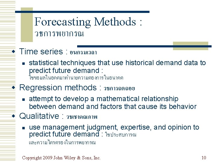
Forecasting Methods : วธการพยากรณ w Time series : อนกรมเวลา n statistical techniques that use historical demand data to predict future demand : ใชขอมลในอดตมาทำนายความตองการในอนาคต w Regression methods : วธการถดถอย n attempt to develop a mathematical relationship between demand factors that cause its behavior w Qualitative : วธเชงคณภาพ n use management judgment, expertise, and opinion to predict future demand : ใชประสบการณ และความไตรตรองในการพยากรณ Copyright 2009 John Wiley & Sons, Inc. 10

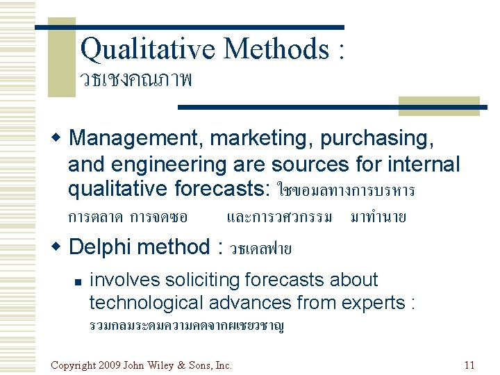
Qualitative Methods : วธเชงคณภาพ w Management, marketing, purchasing, and engineering are sources for internal qualitative forecasts: ใชขอมลทางการบรหาร การตลาด การจดซอ และการวศวกรรม มาทำนาย w Delphi method : วธเดลฟาย n involves soliciting forecasts about technological advances from experts : รวมกลมระดมความคดจากผเชยวชาญ Copyright 2009 John Wiley & Sons, Inc. 11

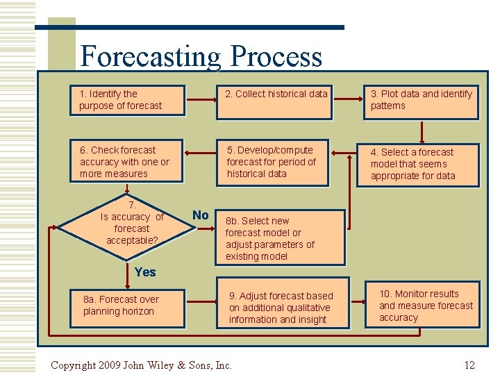
Forecasting Process 1. Identify the purpose of forecast 2. Collect historical data 3. Plot data and identify patterns 6. Check forecast accuracy with one or more measures 5. Develop/compute forecast for period of historical data 4. Select a forecast model that seems appropriate for data 7. Is accuracy of forecast acceptable? No 8 b. Select new forecast model or adjust parameters of existing model Yes 8 a. Forecast over planning horizon 9. Adjust forecast based on additional qualitative information and insight Copyright 2009 John Wiley & Sons, Inc. 10. Monitor results and measure forecast accuracy 12

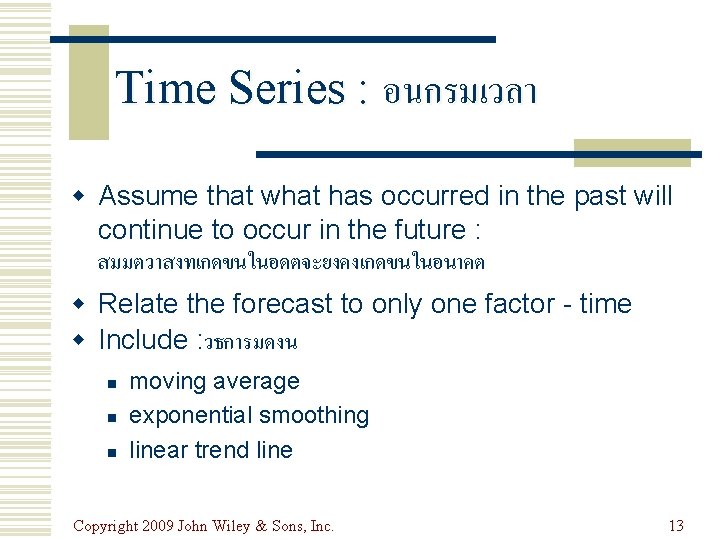
Time Series : อนกรมเวลา w Assume that what has occurred in the past will continue to occur in the future : สมมตวาสงทเกดขนในอดตจะยงคงเกดขนในอนาคต w Relate the forecast to only one factor - time w Include : วธการมดงน n n n moving average exponential smoothing linear trend line Copyright 2009 John Wiley & Sons, Inc. 13

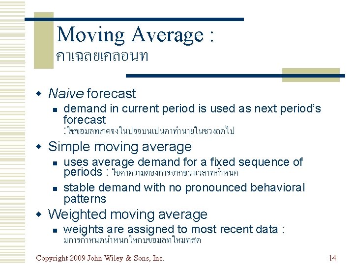
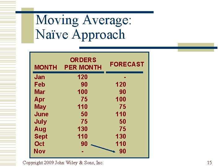
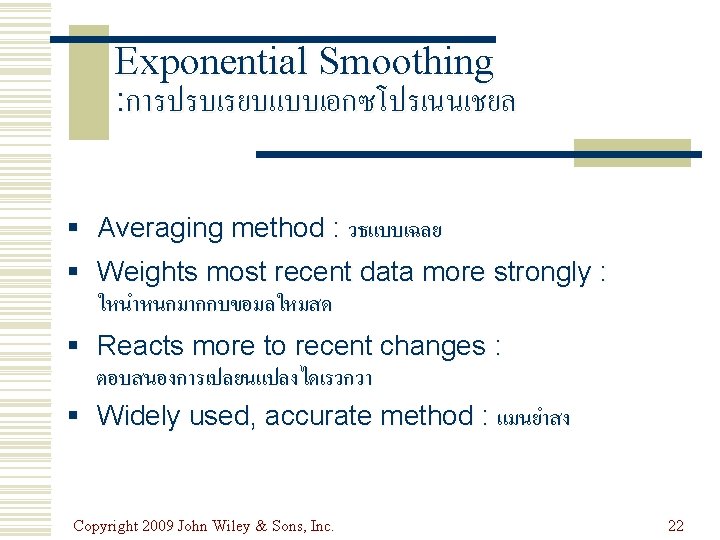
Moving Average : คาเฉลยเคลอนท w Naive forecast n demand in current period is used as next period’s forecast : ใชขอมลทเกดจงในปจจบนเปนคาทำนายในชวงถดไป w Simple moving average n n uses average demand for a fixed sequence of periods : ใชคาความตองการจากชวงเวลาทกำหนด stable demand with no pronounced behavioral patterns w Weighted moving average n weights are assigned to most recent data : มการกำหนดนำหนกใหกบขอมลทใหมทสด Copyright 2009 John Wiley & Sons, Inc. 14

Moving Average: Naïve Approach MONTH Jan Feb Mar Apr May June July Aug Sept Oct Nov ORDERS PER MONTH 120 90 100 75 110 50 75 130 110 90 - Copyright 2009 John Wiley & Sons, Inc. FORECAST 120 90 100 75 110 50 75 130 110 90 15

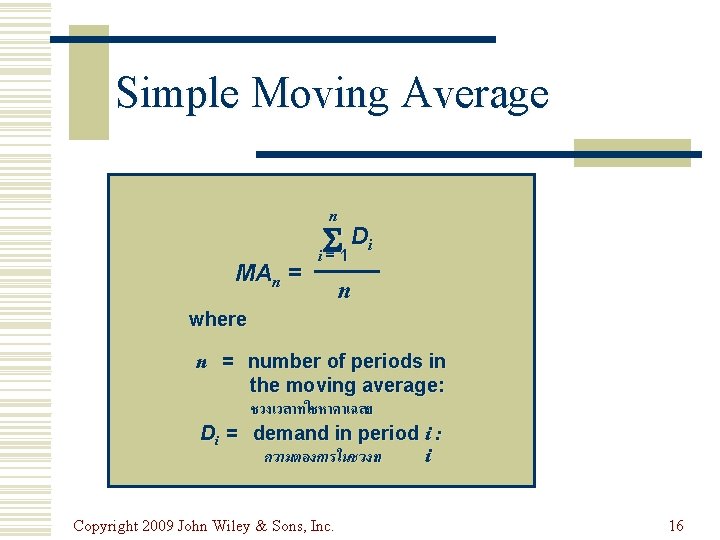
Simple Moving Average n MAn = Di i=1 n where n = number of periods in the moving average: ชวงเวลาทใชหาคาเฉลย Di = demand in period i : ความตองการในชวงท i Copyright 2009 John Wiley & Sons, Inc. 16

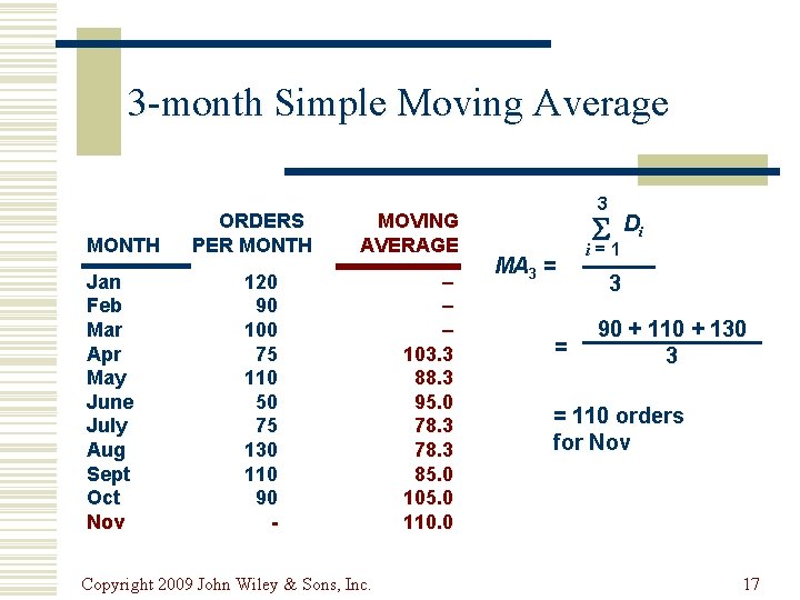
3 -month Simple Moving Average MONTH Jan Feb Mar Apr May June July Aug Sept Oct Nov ORDERS PER MONTH MOVING AVERAGE 120 90 100 75 110 50 75 130 110 90 - Copyright 2009 John Wiley & Sons, Inc. – – – 103. 3 88. 3 95. 0 78. 3 85. 0 105. 0 110. 0 3 MA 3 = = Di i=1 3 90 + 110 + 130 3 = 110 orders for Nov 17

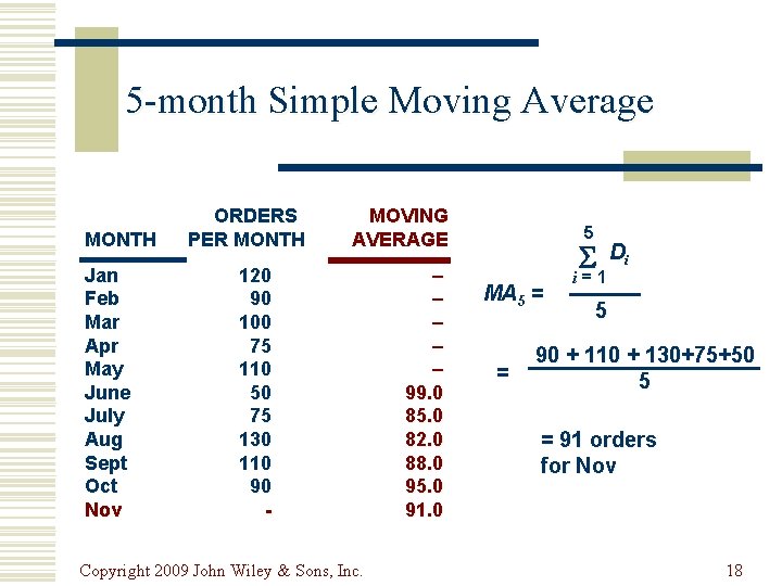
5 -month Simple Moving Average MONTH Jan Feb Mar Apr May June July Aug Sept Oct Nov ORDERS PER MONTH MOVING AVERAGE 120 90 100 75 110 50 75 130 110 90 - Copyright 2009 John Wiley & Sons, Inc. – – – 99. 0 85. 0 82. 0 88. 0 95. 0 91. 0 5 MA 5 = = Di i=1 5 90 + 110 + 130+75+50 5 = 91 orders for Nov 18

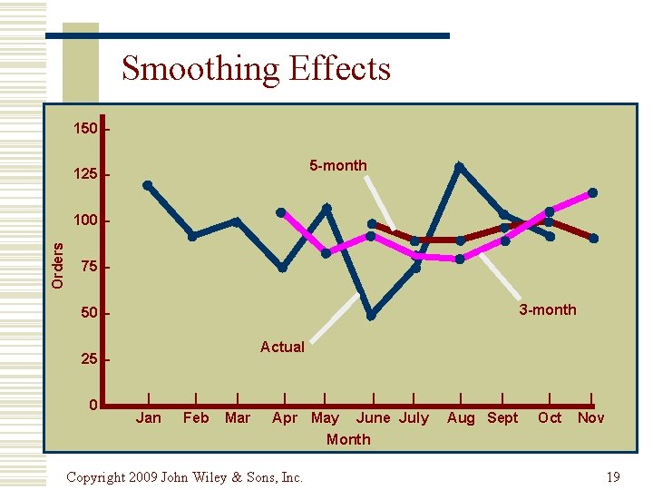
Smoothing Effects 150 – 5 -month 125 – Orders 100 – 75 – 3 -month 50 – Actual 25 – 0– | Jan | Feb | Mar | | Apr May June July Month Copyright 2009 John Wiley & Sons, Inc. | | Aug Sept | Oct | Nov 19

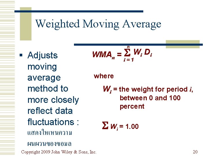
Weighted Moving Average n § Adjusts moving average method to more closely reflect data fluctuations : แสดงใหเหนความ ผนผวนของขอมล WMAn = Wi Di i=1 where Copyright 2009 John Wiley & Sons, Inc. Wi = the weight for period i, between 0 and 100 percent Wi = 1. 00 20

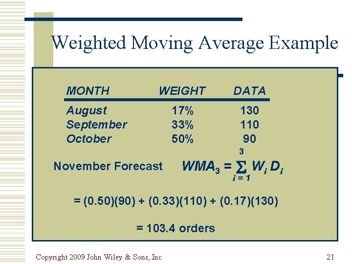
Weighted Moving Average Example MONTH WEIGHT DATA 17% 33% 50% 130 110 90 August September October 3 November Forecast WMA 3 = Wi Di i=1 = (0. 50)(90) + (0. 33)(110) + (0. 17)(130) = 103. 4 orders Copyright 2009 John Wiley & Sons, Inc. 21

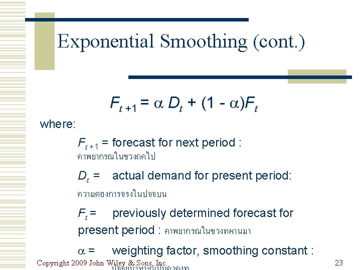
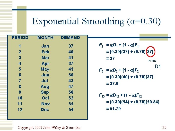
Exponential Smoothing (cont. ) Ft +1 = Dt + (1 - )Ft where: Ft +1 = forecast for next period : คาพยากรณในชวงถดไป Dt = actual demand for present period: ความตองการจรงในปจจบน Ft = previously determined forecast for present period : คาพยากรณในชวงทผานมา = weighting factor, smoothing constant : Copyright 2009 John Wiley & Sons, Inc. 23

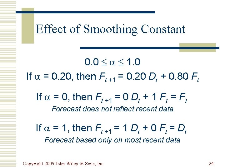
Effect of Smoothing Constant 0. 0 1. 0 If = 0. 20, then Ft +1 = 0. 20 Dt + 0. 80 Ft If = 0, then Ft +1 = 0 Dt + 1 Ft = Ft Forecast does not reflect recent data If = 1, then Ft +1 = 1 Dt + 0 Ft = Dt Forecast based only on most recent data Copyright 2009 John Wiley & Sons, Inc. 24

Exponential Smoothing (α=0. 30) PERIOD MONTH DEMAND 1 2 3 4 5 6 7 8 9 10 11 12 Jan Feb Mar Apr May Jun Jul Aug Sep Oct Nov Dec 37 40 41 37 45 50 43 47 56 52 55 54 Copyright 2009 John Wiley & Sons, Inc. F 2 = D 1 + (1 - )F 1 = (0. 30)(37) + (0. 70)(37) = 37 F 3 = D 2 + (1 - )F 2 เทากบ D 1 = (0. 30)(40) + (0. 70)(37) = 37. 9 F 13 = D 12 + (1 - )F 12 = (0. 30)(54) + (0. 70)(50. 84) = 51. 79 25

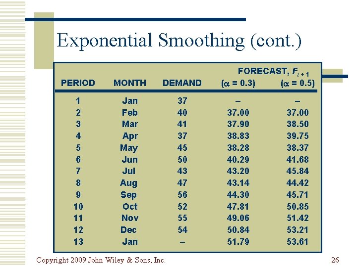
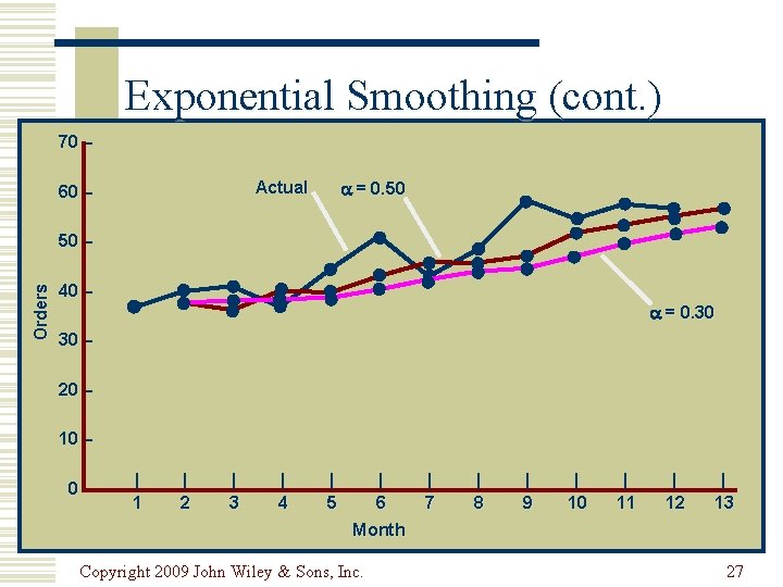
Exponential Smoothing (cont. ) PERIOD MONTH DEMAND 1 2 3 4 5 6 7 8 9 10 11 12 13 Jan Feb Mar Apr May Jun Jul Aug Sep Oct Nov Dec Jan 37 40 41 37 45 50 43 47 56 52 55 54 – Copyright 2009 John Wiley & Sons, Inc. FORECAST, Ft + 1 ( = 0. 3) ( = 0. 5) – 37. 00 37. 90 38. 83 38. 28 40. 29 43. 20 43. 14 44. 30 47. 81 49. 06 50. 84 51. 79 – 37. 00 38. 50 39. 75 38. 37 41. 68 45. 84 44. 42 45. 71 50. 85 51. 42 53. 21 53. 61 26

Exponential Smoothing (cont. ) 70 – = 0. 50 Actual 60 – Orders 50 – 40 – = 0. 30 30 – 20 – 10 – 0– | 1 | 2 | 3 | 4 | 5 | 6 | 7 | 8 | 9 | 10 | 11 | 12 | 13 Month Copyright 2009 John Wiley & Sons, Inc. 27

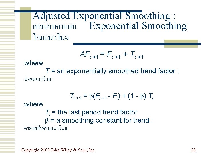
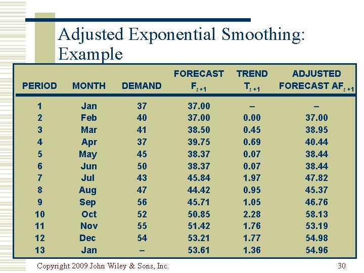
Adjusted Exponential Smoothing : การปรบคาแบบ Exponential Smoothing โยมแนวโนม where AFt +1 = Ft +1 + Tt +1 T = an exponentially smoothed trend factor : ปจจยแนวโนม where Tt +1 = (Ft +1 - Ft) + (1 - ) Tt Tt = the last period trend factor = a smoothing constant for trend : คาคงทสำหรบแนวโนม Copyright 2009 John Wiley & Sons, Inc. 28

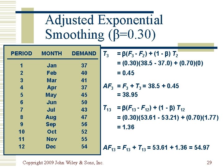
Adjusted Exponential Smoothing (β=0. 30) PERIOD MONTH DEMAND 1 2 3 4 5 6 7 8 9 10 11 12 Jan Feb Mar Apr May Jun Jul Aug Sep Oct Nov Dec 37 40 41 37 45 50 43 47 56 52 55 54 T 3 = (F 3 - F 2) + (1 - ) T 2 = (0. 30)(38. 5 - 37. 0) + (0. 70)(0) = 0. 45 AF 3 = F 3 + T 3 = 38. 5 + 0. 45 = 38. 95 T 13 = (F 13 - F 12) + (1 - ) T 12 = (0. 30)(53. 61 - 53. 21) + (0. 70)(1. 77) = 1. 36 AF 13 = F 13 + T 13 = 53. 61 + 1. 36 = 54. 97 Copyright 2009 John Wiley & Sons, Inc. 29

Adjusted Exponential Smoothing: Example PERIOD MONTH DEMAND FORECAST Ft +1 1 2 3 4 5 6 7 8 9 10 11 12 13 Jan Feb Mar Apr May Jun Jul Aug Sep Oct Nov Dec Jan 37 40 41 37 45 50 43 47 56 52 55 54 – 37. 00 38. 50 39. 75 38. 37 45. 84 44. 42 45. 71 50. 85 51. 42 53. 21 53. 61 Copyright 2009 John Wiley & Sons, Inc. TREND Tt +1 ADJUSTED FORECAST AFt +1 – 0. 00 0. 45 0. 69 0. 07 1. 97 0. 95 1. 05 2. 28 1. 76 1. 77 1. 36 – 37. 00 38. 95 40. 44 38. 44 47. 82 45. 37 46. 76 58. 13 53. 19 54. 98 54. 96 30

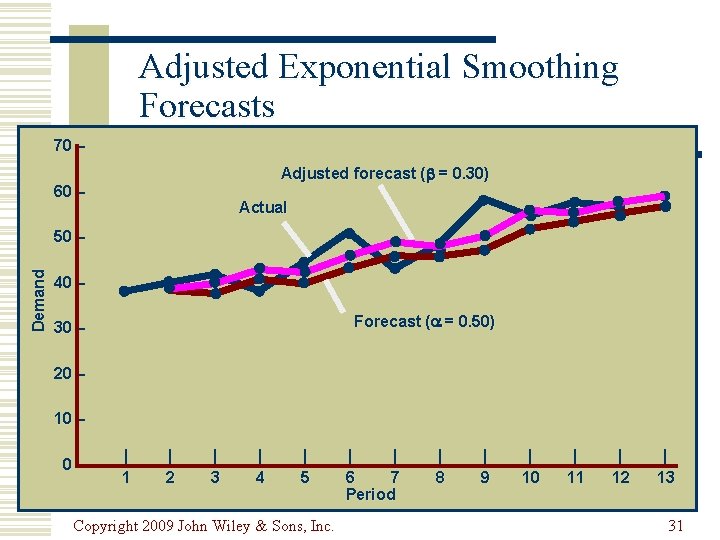
Adjusted Exponential Smoothing Forecasts 70 – Adjusted forecast ( = 0. 30) 60 – Actual Demand 50 – 40 – Forecast ( = 0. 50) 30 – 20 – 10 – 0– | 1 | 2 | 3 | 4 | 5 Copyright 2009 John Wiley & Sons, Inc. | | 6 7 Period | 8 | 9 | 10 | 11 | 12 | 13 31

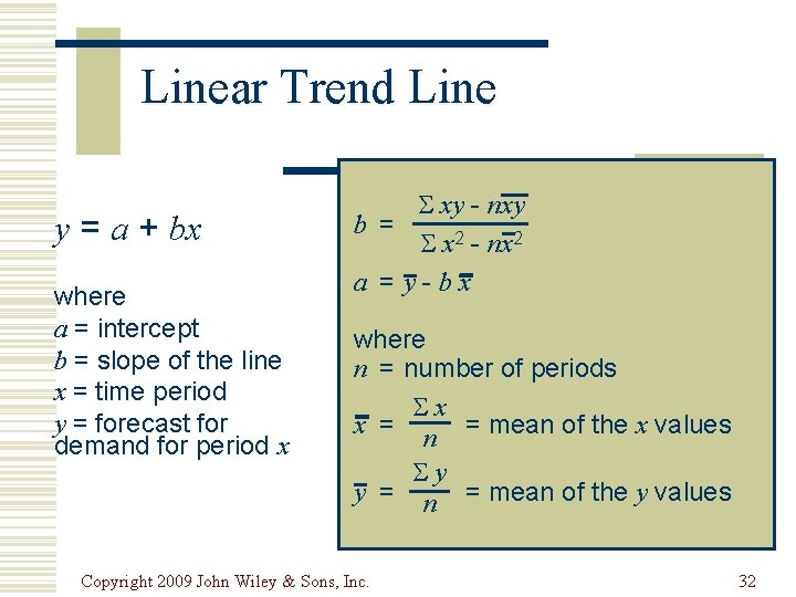
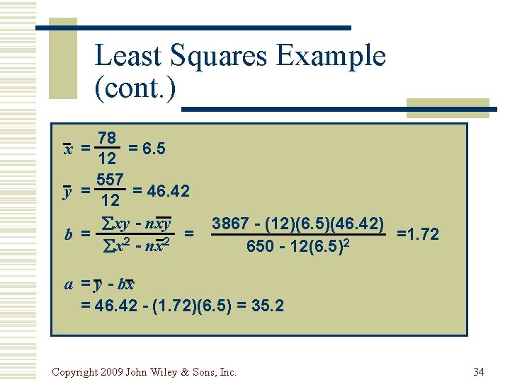
Linear Trend Line y = a + bx where a = intercept b = slope of the line x = time period y = forecast for demand for period x xy - nxy b = x 2 - nx 2 a = y-bx where n = number of periods x x = n = mean of the x values y y = n = mean of the y values Copyright 2009 John Wiley & Sons, Inc. 32

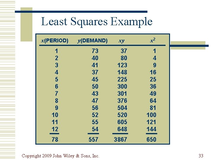
Least Squares Example x(PERIOD) y(DEMAND) xy x 2 1 2 3 4 5 6 7 8 9 10 11 12 73 40 41 37 45 50 43 47 56 52 55 54 37 80 123 148 225 300 301 376 504 520 605 648 1 4 9 16 25 36 49 64 81 100 121 144 78 557 3867 650 Copyright 2009 John Wiley & Sons, Inc. 33

Least Squares Example (cont. ) 78 x = = 6. 5 12 557 y = = 46. 42 12 xy - nxy b = = 2 2 x - nx 3867 - (12)(6. 5)(46. 42) =1. 72 2 650 - 12(6. 5) a = y - bx = 46. 42 - (1. 72)(6. 5) = 35. 2 Copyright 2009 John Wiley & Sons, Inc. 34

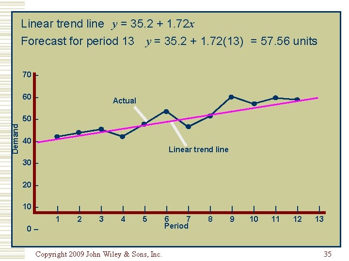
Linear trend line y = 35. 2 + 1. 72 x Forecast for period 13 y = 35. 2 + 1. 72(13) = 57. 56 units 70 – Demand 60 – Actual 50 – 40 – Linear trend line 30 – 20 – 10 – | 1 | 2 | 3 | 4 | 5 0– Copyright 2009 John Wiley & Sons, Inc. | | 6 7 Period | 8 | 9 | 10 | 11 | 12 | 13 35

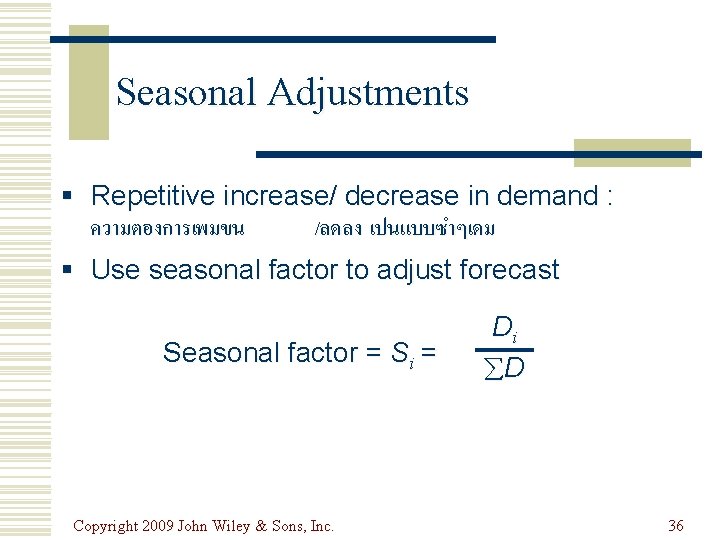
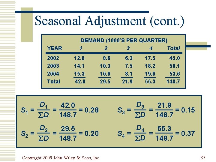
Seasonal Adjustments § Repetitive increase/ decrease in demand : ความตองการเพมขน /ลดลง เปนแบบซำๆเดม § Use seasonal factor to adjust forecast Seasonal factor = Si = Copyright 2009 John Wiley & Sons, Inc. Di D 36

Seasonal Adjustment (cont. ) YEAR 2002 2003 2004 Total DEMAND (1000’S PER QUARTER) 1 2 3 4 Total 12. 6 14. 1 15. 3 42. 0 8. 6 10. 3 10. 6 29. 5 6. 3 7. 5 8. 1 21. 9 17. 5 18. 2 19. 6 55. 3 45. 0 50. 1 53. 6 148. 7 D 1 42. 0 S 1 = = = 0. 28 D 148. 7 D 3 21. 9 S 3 = = = 0. 15 D 148. 7 D 2 29. 5 S 2 = = = 0. 20 D 148. 7 D 4 55. 3 S 4 = = = 0. 37 D 148. 7 Copyright 2009 John Wiley & Sons, Inc. 37

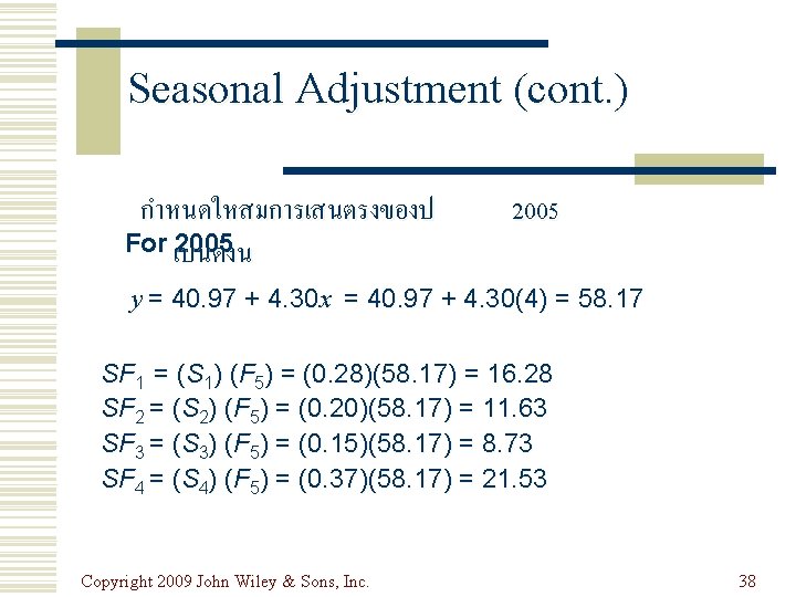
Seasonal Adjustment (cont. ) กำหนดใหสมการเสนตรงของป For เปนดงน 2005 y = 40. 97 + 4. 30 x = 40. 97 + 4. 30(4) = 58. 17 SF 1 = (S 1) (F 5) = (0. 28)(58. 17) = 16. 28 SF 2 = (S 2) (F 5) = (0. 20)(58. 17) = 11. 63 SF 3 = (S 3) (F 5) = (0. 15)(58. 17) = 8. 73 SF 4 = (S 4) (F 5) = (0. 37)(58. 17) = 21. 53 Copyright 2009 John Wiley & Sons, Inc. 38

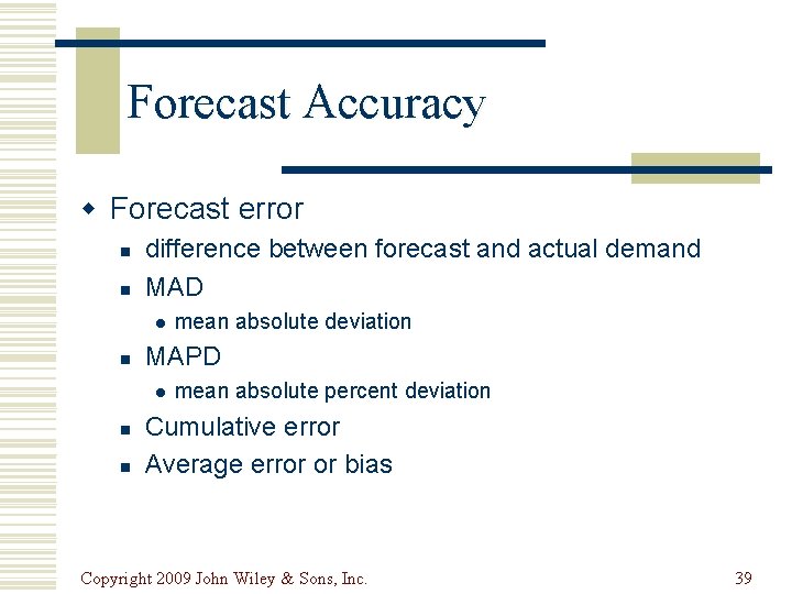
Forecast Accuracy w Forecast error n n difference between forecast and actual demand MAD l n MAPD l n n mean absolute deviation mean absolute percent deviation Cumulative error Average error or bias Copyright 2009 John Wiley & Sons, Inc. 39

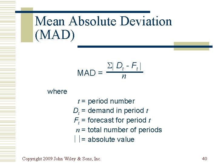
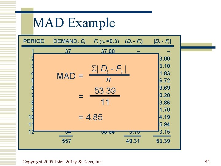
Mean Absolute Deviation (MAD) Dt - F t MAD = n where t = period number Dt = demand in period t Ft = forecast for period t n = total number of periods = absolute value Copyright 2009 John Wiley & Sons, Inc. 40

MAD Example PERIOD 1 2 3 4 5 6 7 8 9 10 11 12 DEMAND, Dt 37 40 41 37 MAD 45 50 43 47 56 52 55 54 = = = Ft ( =0. 3) (Dt - Ft) |Dt - Ft| 37. 00 – 37. 00 37. 90 3. 10 D F t t -1. 83 38. 83 n 38. 28 6. 72 40. 29 9. 69 53. 39 43. 20 -0. 20 43. 14 3. 86 11 44. 30 11. 70 4. 19 4. 8547. 81 49. 06 5. 94 50. 84 3. 15 – 3. 00 3. 10 1. 83 6. 72 9. 69 0. 20 3. 86 11. 70 4. 19 5. 94 3. 15 49. 31 53. 39 557 Copyright 2009 John Wiley & Sons, Inc. 41

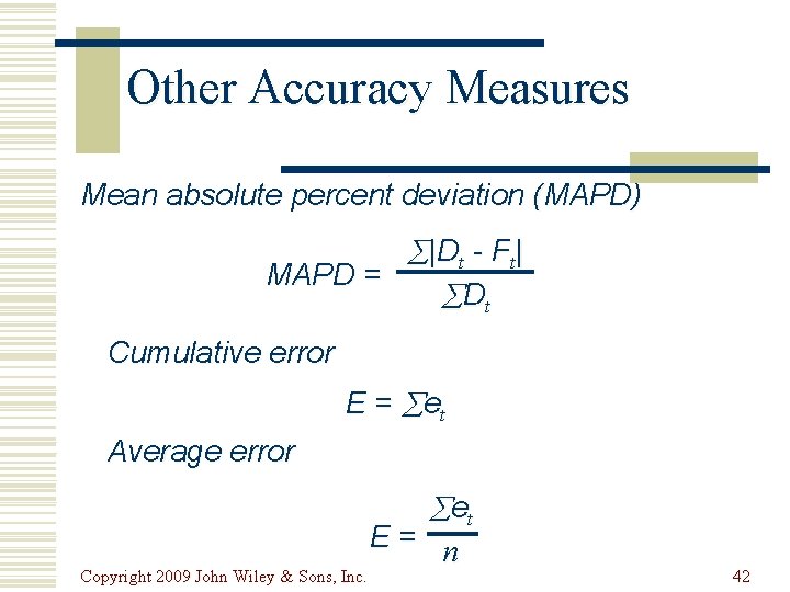
Other Accuracy Measures Mean absolute percent deviation (MAPD) |Dt - Ft| MAPD = Dt Cumulative error E = et Average error et Copyright 2009 John Wiley & Sons, Inc. E= n 42

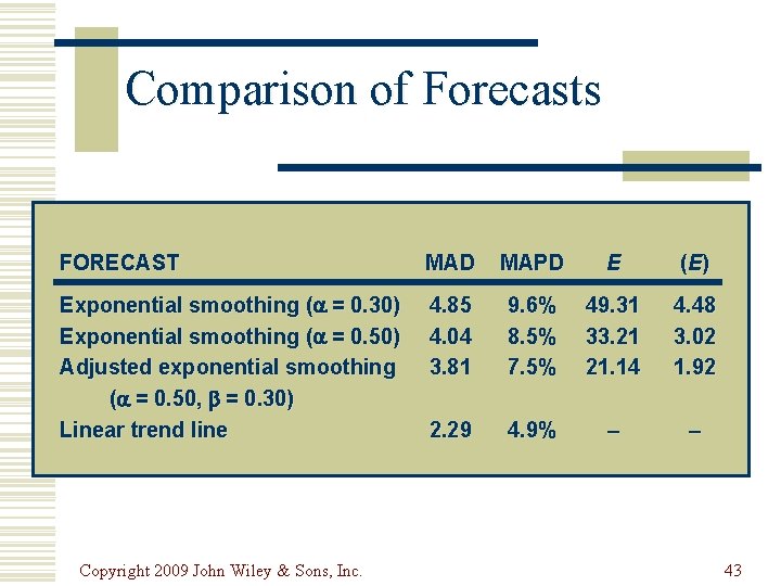
Comparison of Forecasts FORECAST MAD MAPD E (E ) Exponential smoothing ( = 0. 30) Exponential smoothing ( = 0. 50) Adjusted exponential smoothing ( = 0. 50, = 0. 30) Linear trend line 4. 85 4. 04 3. 81 9. 6% 8. 5% 7. 5% 49. 31 33. 21 21. 14 4. 48 3. 02 1. 92 2. 29 4. 9% – – Copyright 2009 John Wiley & Sons, Inc. 43

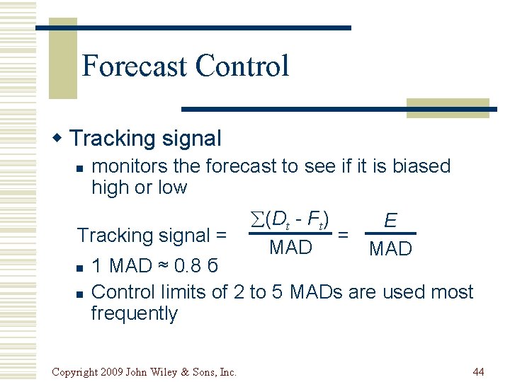
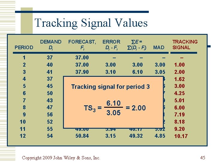
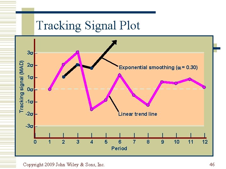
Forecast Control w Tracking signal n monitors the forecast to see if it is biased high or low (D t - F t ) E = MAD Tracking signal = n 1 MAD ≈ 0. 8 б n Control limits of 2 to 5 MADs are used most frequently Copyright 2009 John Wiley & Sons, Inc. 44

Tracking Signal Values PERIOD DEMAND Dt 1 2 3 4 5 6 7 8 9 10 11 12 37 40 41 37 45 50 43 47 56 52 55 54 FORECAST, Ft ERROR Dt - F t E = (Dt - Ft) 37. 00 – – 37. 00 37. 90 3. 10 6. 10 38. 83 -1. 83 4. 27 38. 28 6. 72 for period 10. 99 3 Tracking signal 40. 29 9. 69 20. 68 43. 20 -0. 20 6. 10 20. 48 43. 14 TS 3 = 3. 86 =24. 34 2. 00 3. 05 36. 04 44. 30 11. 70 47. 81 4. 19 40. 23 49. 06 5. 94 46. 17 50. 84 3. 15 49. 32 Copyright 2009 John Wiley & Sons, Inc. MAD – 3. 00 3. 05 2. 64 3. 66 4. 87 4. 09 4. 06 5. 01 4. 92 5. 02 4. 85 TRACKING SIGNAL – 1. 00 2. 00 1. 62 3. 00 4. 25 5. 01 6. 00 7. 19 8. 18 9. 20 10. 17 45

Tracking Signal Plot Tracking signal (MAD) 3 – 2 – Exponential smoothing ( = 0. 30) 1 – 0 – -1 – -2 – Linear trend line -3 – | 0 | 1 | 2 | 3 | 4 | 5 Copyright 2009 John Wiley & Sons, Inc. | 6 Period | 7 | 8 | 9 | 10 | 11 | 12 46

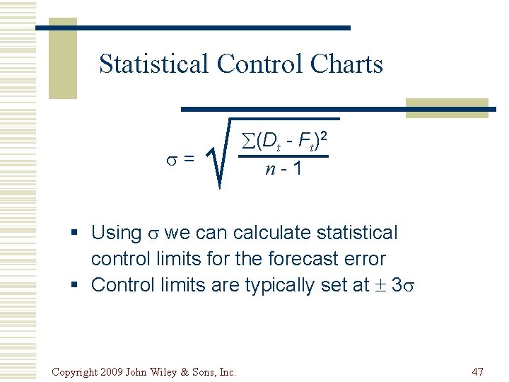
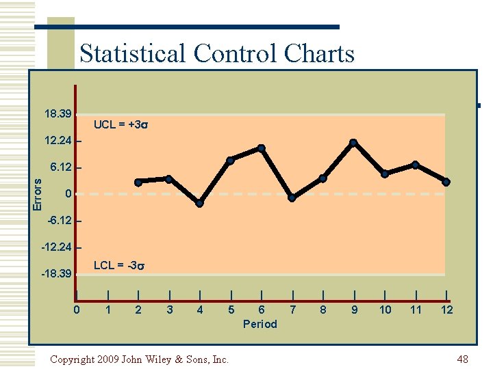
Statistical Control Charts = (D t - F t )2 n-1 § Using we can calculate statistical control limits for the forecast error § Control limits are typically set at 3 Copyright 2009 John Wiley & Sons, Inc. 47

Statistical Control Charts 18. 39 – UCL = +3 12. 24 – Errors 6. 12 – 0– -6. 12 – -12. 24 – -18. 39 – | 0 LCL = -3 | 1 | 2 | 3 | 4 | 5 Copyright 2009 John Wiley & Sons, Inc. | 6 Period | 7 | 8 | 9 | 10 | 11 | 12 48

Time Series Forecasting using Excel w Excel can be used to develop forecasts: n n Moving average Exponential smoothing Adjusted exponential smoothing Linear trend line Copyright 2009 John Wiley & Sons, Inc. 49

Exponentially Smoothed and Adjusted Exponentially Smoothed Forecasts w Insert Exhibit 12. 1 Copyright 2009 John Wiley & Sons, Inc. 50

Demand exponentially smoothed forecast w Insert Exhibit 12. 2 Copyright 2009 John Wiley & Sons, Inc. 51

Data Analysis option w Insert Exhibit 12. 3 w Insert Exhibit 12. 4 Copyright 2009 John Wiley & Sons, Inc. 52

Computing a Forecast with Seasonal Adjustment w Insert Exhibit 12. 5 Copyright 2009 John Wiley & Sons, Inc. 53

OM Tools w Insert Exhibit 12. 6 Copyright 2009 John Wiley & Sons, Inc. 54

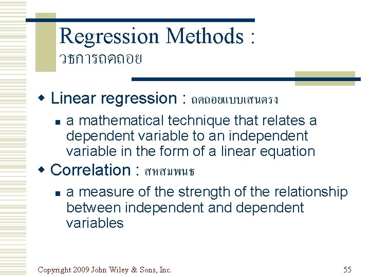
Regression Methods : วธการถดถอย w Linear regression : ถดถอยแบบเสนตรง n a mathematical technique that relates a dependent variable to an independent variable in the form of a linear equation w Correlation : สหสมพนธ n a measure of the strength of the relationship between independent and dependent variables Copyright 2009 John Wiley & Sons, Inc. 55

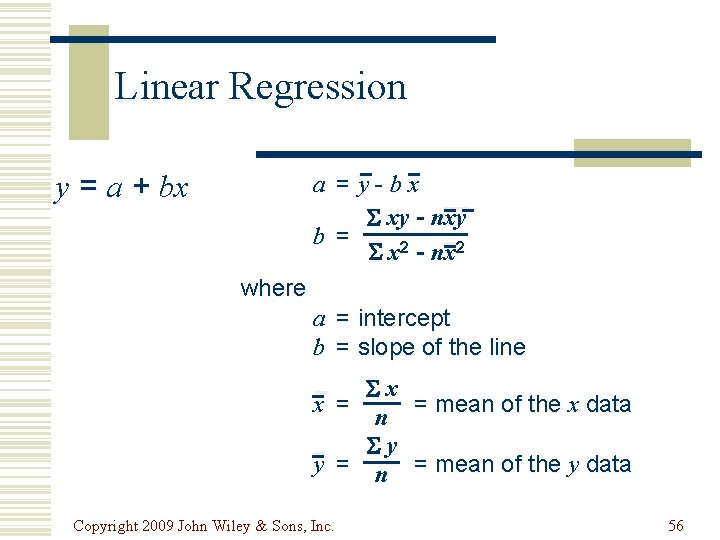
Linear Regression y = a + bx a = y-bx xy - nxy b = x 2 - nx 2 where a = intercept b = slope of the line x x = = mean of the x data n y y = n = mean of the y data Copyright 2009 John Wiley & Sons, Inc. 56

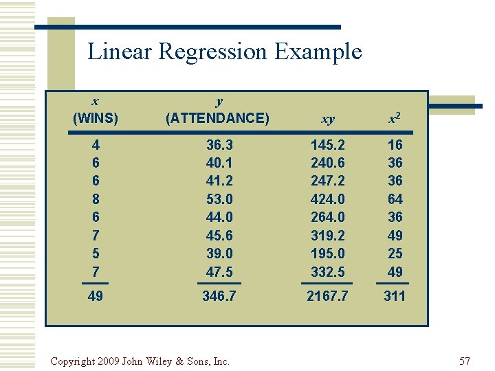
Linear Regression Example x (WINS) y (ATTENDANCE) xy x 2 4 6 6 8 6 7 5 7 36. 3 40. 1 41. 2 53. 0 44. 0 45. 6 39. 0 47. 5 145. 2 240. 6 247. 2 424. 0 264. 0 319. 2 195. 0 332. 5 16 36 36 64 36 49 25 49 49 346. 7 2167. 7 311 Copyright 2009 John Wiley & Sons, Inc. 57

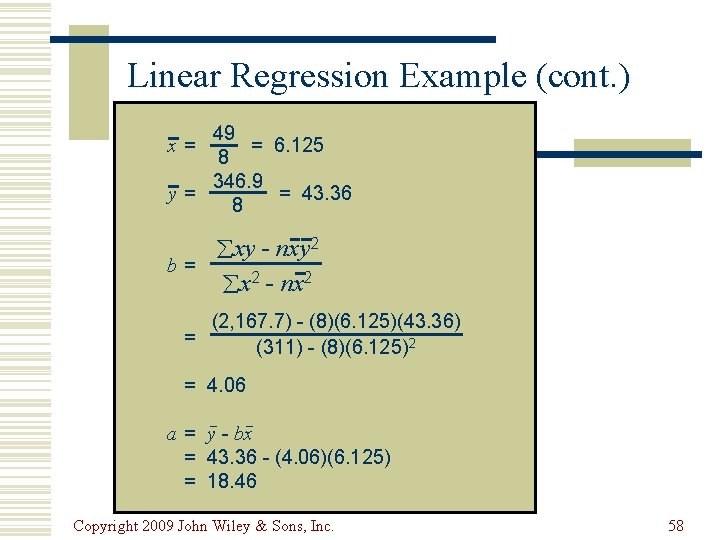
Linear Regression Example (cont. ) 49 = 6. 125 8 346. 9 y= = 43. 36 8 x= xy - nxy 2 b= x 2 - nx 2 (2, 167. 7) - (8)(6. 125)(43. 36) = (311) - (8)(6. 125)2 = 4. 06 a = y - bx = 43. 36 - (4. 06)(6. 125) = 18. 46 Copyright 2009 John Wiley & Sons, Inc. 58

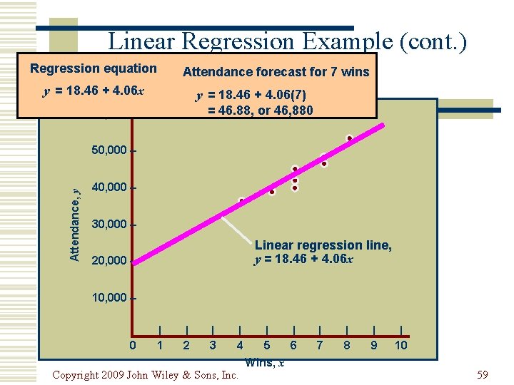
Linear Regression Example (cont. ) Regression equation Attendance forecast for 7 wins y = 18. 46 + 4. 06 x y = 18. 46 + 4. 06(7) = 46. 88, or 46, 880 60, 000 – Attendance, y 50, 000 – 40, 000 – 30, 000 – Linear regression line, y = 18. 46 + 4. 06 x 20, 000 – 10, 000 – | 0 | 1 | 2 | 3 | 4 Copyright 2009 John Wiley & Sons, Inc. | | 5 6 Wins, x | 7 | 8 | 9 | 10 59

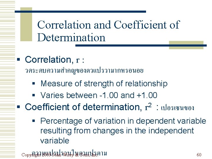
Correlation and Coefficient of Determination § Correlation, r : วดระดบความสำคญของตวแปรวามากหรอนอย § Measure of strength of relationship § Varies between -1. 00 and +1. 00 § Coefficient of determination, r 2 : เปอรเซนของ § Percentage of variation in dependent variable resulting from changes in the independent variable ความแปรปรวนในตวแปรตาม Copyright 2009 John Wiley & Sons, Inc. 60

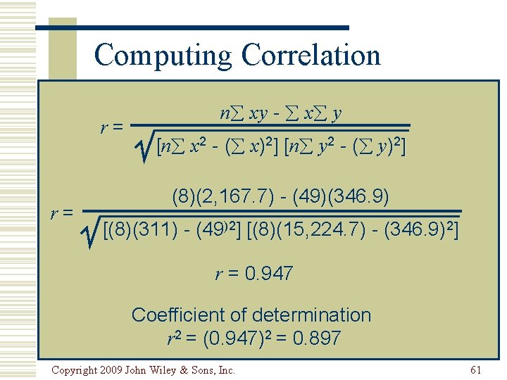
Computing Correlation r= r= n xy - x y [n x 2 - ( x)2] [n y 2 - ( y)2] (8)(2, 167. 7) - (49)(346. 9) [(8)(311) - (49)2] [(8)(15, 224. 7) - (346. 9)2] r = 0. 947 Coefficient of determination r 2 = (0. 947)2 = 0. 897 Copyright 2009 John Wiley & Sons, Inc. 61

Regression Analysis with Excel w Insert Exhibit 12. 7 Copyright 2009 John Wiley & Sons, Inc. 62

Regression Analysis with Excel (cont. ) w Insert Exhibit 12. 8 &12. 9 Copyright 2009 John Wiley & Sons, Inc. 63

Regression Analysis with Excel (cont. ) w Insert Exhibit 12. 10 Copyright 2009 John Wiley & Sons, Inc. 64

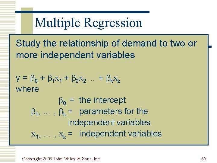
Multiple Regression Study the relationship of demand to two or more independent variables y = 0 + 1 x 1 + 2 x 2 … + kxk where 0 = the intercept 1, … , k = parameters for the independent variables x 1, … , xk = independent variables Copyright 2009 John Wiley & Sons, Inc. 65

Multiple Regression with Excel w Insert Exhibit 12. 11 w Insert Exhibit 12. 12 Copyright 2009 John Wiley & Sons, Inc. 66

Copyright 2009 John Wiley & Sons, Inc. All rights reserved. Reproduction or translation of this work beyond that permitted in section 117 of the 1976 United States Copyright Act without express permission of the copyright owner is unlawful. Request for further information should be addressed to the Permission Department, John Wiley & Sons, Inc. The purchaser may make back-up copies for his/her own use only and not for distribution or resale. The Publisher assumes no responsibility for errors, omissions, or damages caused by the use of these programs or from the use of the information herein. Copyright 2009 John Wiley & Sons, Inc. 67