Chapter 12 Estimating Means with Confidence Copyright 2011

Chapter 12 Estimating Means with Confidence Copyright © 2011 Brooks/Cole, Cengage Learning

11. 1 Introduction to CI for Means • A parameter is a population characteristic – value is usually unknown. We estimate the parameter using sample information. • A statistic, or estimate, is a characteristic of a sample. A statistic estimates a parameter. • A confidence interval is an interval of values computed from sample data that is likely to include the true population value. • The confidence level for an interval describes our confidence in the procedure we used. We are confident that most of the confidence intervals we compute using a procedure will contain the true population value. Copyright © 2011 Brooks/Cole, Cengage Learning 2

More Estimation Situations Situation 1. Estimating the mean of a quantitative variable. Example research questions: What is the mean time that college students watch TV per day? What is the mean pulse rate of women? Population parameter: m (spelled “mu” and pronounced “mew”) = population mean for the variable Sample estimate: = the sample mean for the variable Copyright © 2011 Brooks/Cole, Cengage Learning 3

More Estimation Situations Situation 2. Estimating the population mean of paired differences for a quantitative variable. Example research questions: What is the mean difference in weights for freshmen at the beginning and end of the first semester? What is the mean difference in age between husbands and wives in Britain? Population parameter: md = population mean of the differences in the two measurements Sample estimate: = the mean of the differences for a sample of the two measurements Copyright © 2011 Brooks/Cole, Cengage Learning 4

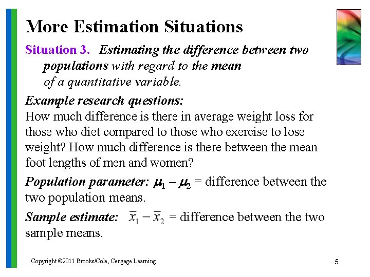
More Estimation Situations Situation 3. Estimating the difference between two populations with regard to the mean of a quantitative variable. Example research questions: How much difference is there in average weight loss for those who diet compared to those who exercise to lose weight? How much difference is there between the mean foot lengths of men and women? Population parameter: m 1 – m 2 = difference between the two population means. Sample estimate: = difference between the two sample means. Copyright © 2011 Brooks/Cole, Cengage Learning 5

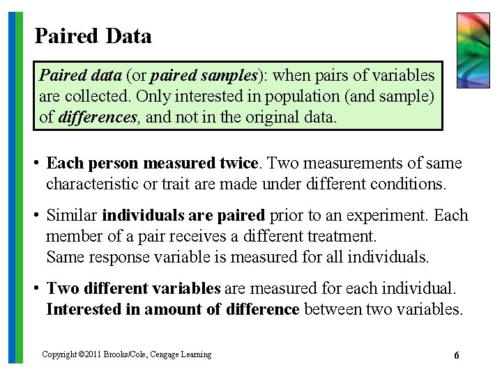
Paired Data Paired data (or paired samples): when pairs of variables are collected. Only interested in population (and sample) of differences, and not in the original data. • Each person measured twice. Two measurements of same characteristic or trait are made under different conditions. • Similar individuals are paired prior to an experiment. Each member of a pair receives a different treatment. Same response variable is measured for all individuals. • Two different variables are measured for each individual. Interested in amount of difference between two variables. Copyright © 2011 Brooks/Cole, Cengage Learning 6

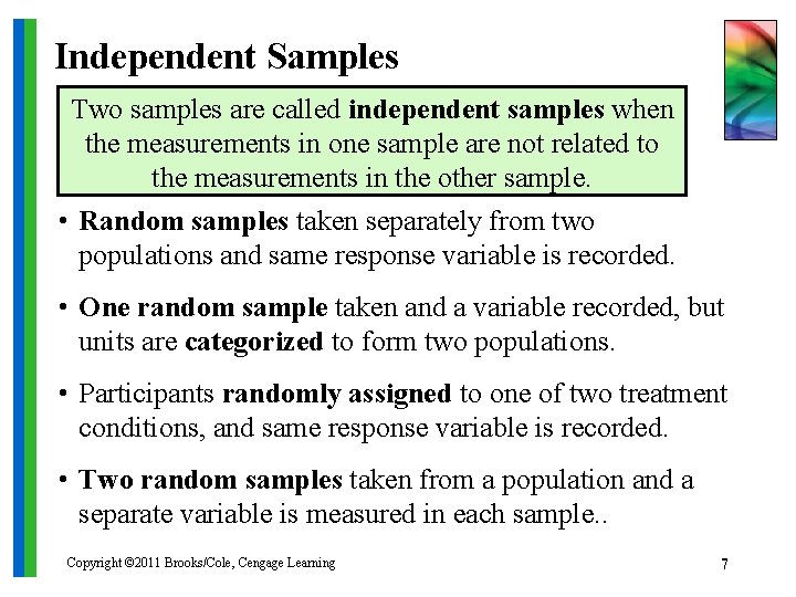
Independent Samples Two samples are called independent samples when the measurements in one sample are not related to the measurements in the other sample. • Random samples taken separately from two populations and same response variable is recorded. • One random sample taken and a variable recorded, but units are categorized to form two populations. • Participants randomly assigned to one of two treatment conditions, and same response variable is recorded. • Two random samples taken from a population and a separate variable is measured in each sample. . Copyright © 2011 Brooks/Cole, Cengage Learning 7

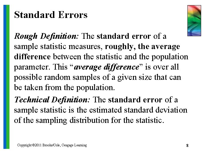
Standard Errors Rough Definition: The standard error of a sample statistic measures, roughly, the average difference between the statistic and the population parameter. This “average difference” is over all possible random samples of a given size that can be taken from the population. Technical Definition: The standard error of a sample statistic is the estimated standard deviation of the sampling distribution for the statistic. Copyright © 2011 Brooks/Cole, Cengage Learning 8

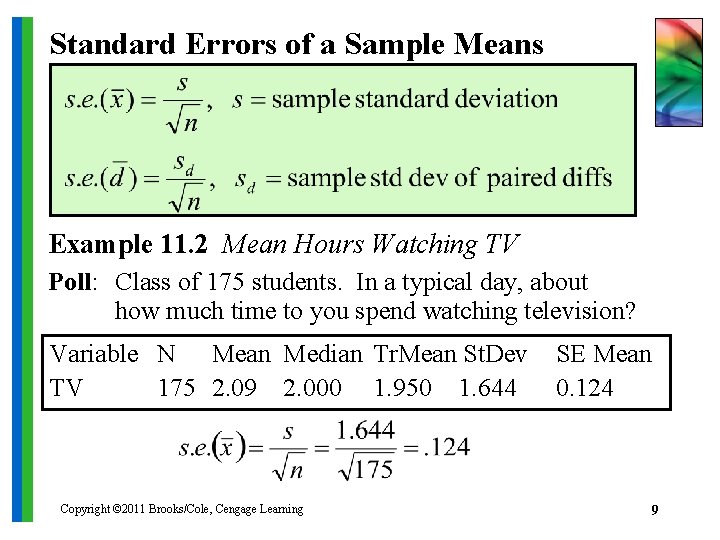
Standard Errors of a Sample Means Example 11. 2 Mean Hours Watching TV Poll: Class of 175 students. In a typical day, about how much time to you spend watching television? Variable N Mean Median Tr. Mean St. Dev TV 175 2. 09 2. 000 1. 950 1. 644 Copyright © 2011 Brooks/Cole, Cengage Learning SE Mean 0. 124 9

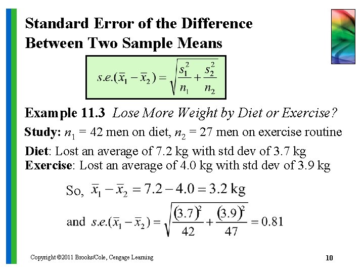
Standard Error of the Difference Between Two Sample Means Example 11. 3 Lose More Weight by Diet or Exercise? Study: n 1 = 42 men on diet, n 2 = 27 men on exercise routine Diet: Lost an average of 7. 2 kg with std dev of 3. 7 kg Exercise: Lost an average of 4. 0 kg with std dev of 3. 9 kg So, Copyright © 2011 Brooks/Cole, Cengage Learning 10

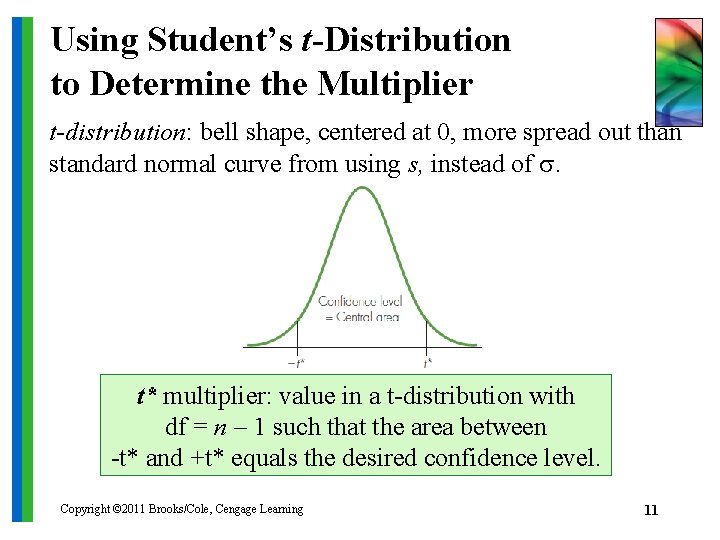
Using Student’s t-Distribution to Determine the Multiplier t-distribution: bell shape, centered at 0, more spread out than standard normal curve from using s, instead of s. t* multiplier: value in a t-distribution with df = n – 1 such that the area between -t* and +t* equals the desired confidence level. Copyright © 2011 Brooks/Cole, Cengage Learning 11

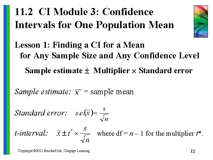
11. 2 CI Module 3: Confidence Intervals for One Population Mean Lesson 1: Finding a CI for a Mean for Any Sample Size and Any Confidence Level Sample estimate Multiplier Standard error Sample estimate: = sample mean Standard error: t-interval: Copyright © 2011 Brooks/Cole, Cengage Learning where df = n – 1 for the multiplier t*. 12

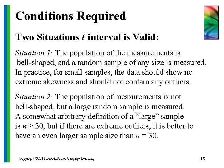
Conditions Required Two Situations t-interval is Valid: Situation 1: The population of the measurements is |bell-shaped, and a random sample of any size is measured. In practice, for small samples, the data should show no extreme skewness and should not contain any outliers. Situation 2: The population of measurements is not bell-shaped, but a large random sample is measured. A somewhat arbitrary definition of a “large” sample is n ≥ 30, but if there are extreme outliers, it is better to have an even larger sample size than n = 30. Copyright © 2011 Brooks/Cole, Cengage Learning 13

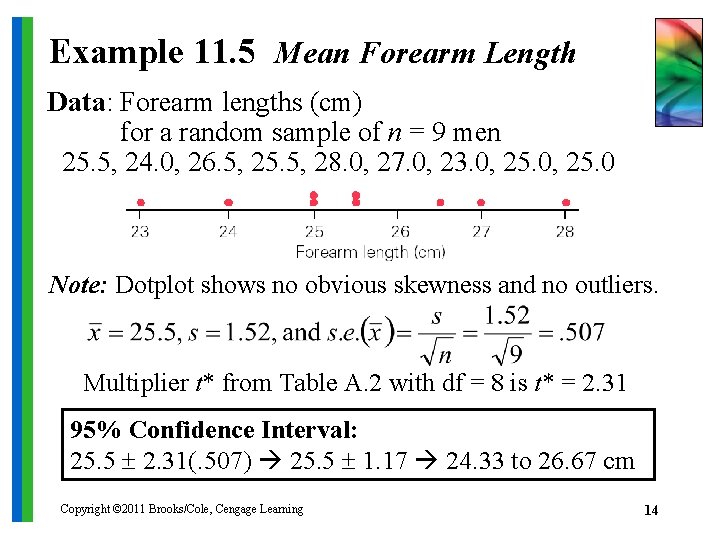
Example 11. 5 Mean Forearm Length Data: Forearm lengths (cm) for a random sample of n = 9 men 25. 5, 24. 0, 26. 5, 25. 5, 28. 0, 27. 0, 23. 0, 25. 0 Note: Dotplot shows no obvious skewness and no outliers. Multiplier t* from Table A. 2 with df = 8 is t* = 2. 31 95% Confidence Interval: 25. 5 2. 31(. 507) 25. 5 1. 17 24. 33 to 26. 67 cm Copyright © 2011 Brooks/Cole, Cengage Learning 14

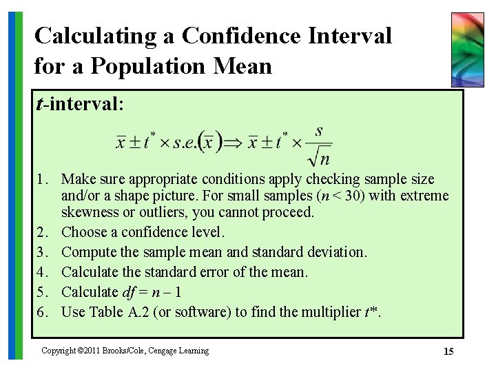
Calculating a Confidence Interval for a Population Mean t-interval: 1. Make sure appropriate conditions apply checking sample size and/or a shape picture. For small samples (n < 30) with extreme skewness or outliers, you cannot proceed. 2. Choose a confidence level. 3. Compute the sample mean and standard deviation. 4. Calculate the standard error of the mean. 5. Calculate df = n – 1 6. Use Table A. 2 (or software) to find the multiplier t*. Copyright © 2011 Brooks/Cole, Cengage Learning 15

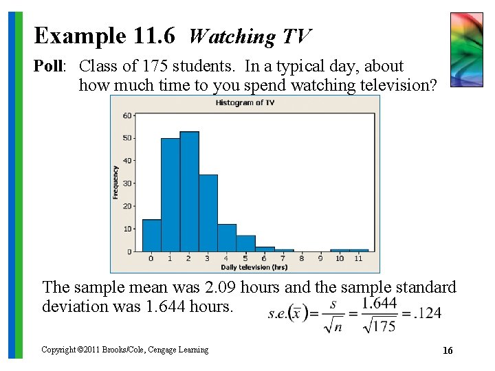
Example 11. 6 Watching TV Poll: Class of 175 students. In a typical day, about how much time to you spend watching television? The sample mean was 2. 09 hours and the sample standard deviation was 1. 644 hours. Copyright © 2011 Brooks/Cole, Cengage Learning 16

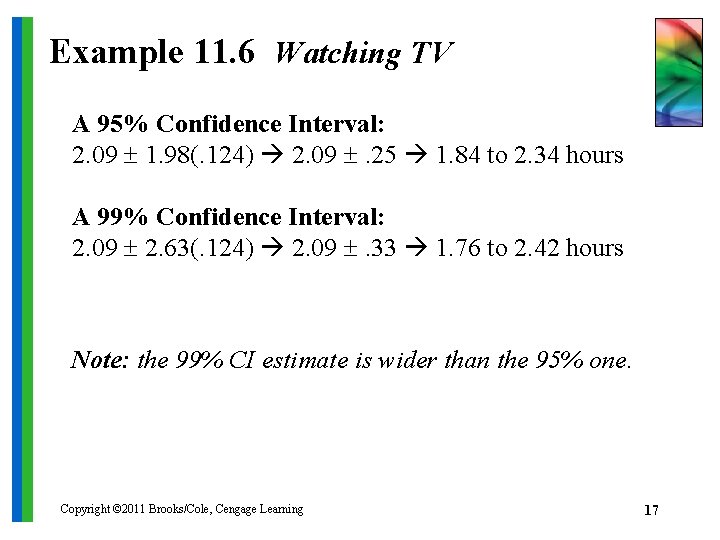
Example 11. 6 Watching TV A 95% Confidence Interval: 2. 09 1. 98(. 124) 2. 09 . 25 1. 84 to 2. 34 hours A 99% Confidence Interval: 2. 09 2. 63(. 124) 2. 09 . 33 1. 76 to 2. 42 hours Note: the 99% CI estimate is wider than the 95% one. Copyright © 2011 Brooks/Cole, Cengage Learning 17

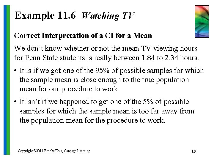
Example 11. 6 Watching TV Correct Interpretation of a CI for a Mean We don’t know whether or not the mean TV viewing hours for Penn State students is really between 1. 84 to 2. 34 hours. • It is if we got one of the 95% of possible samples for which the sample mean is close enough to the true population mean for our procedure to work. • It isn’t if we happened to get one of the 5% of possible samples for which the sample mean is too far away from the population mean for the procedure to work. Copyright © 2011 Brooks/Cole, Cengage Learning 18

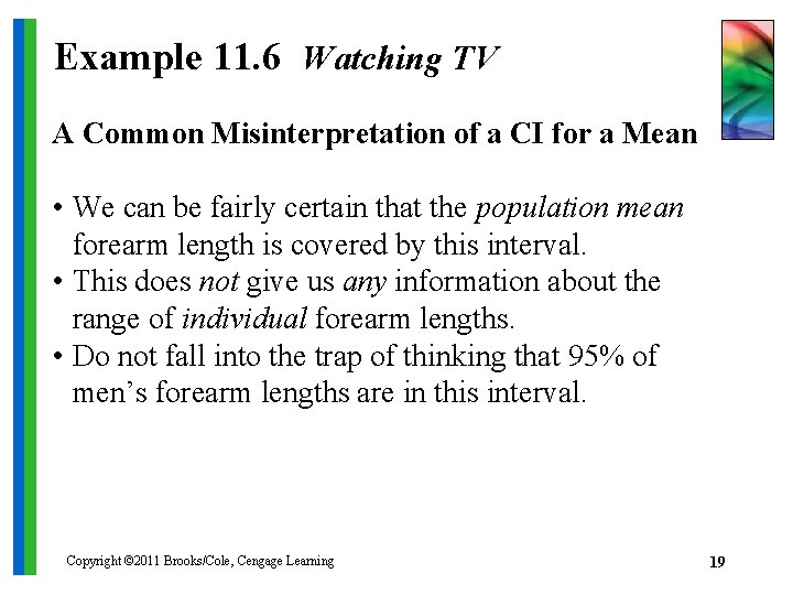
Example 11. 6 Watching TV A Common Misinterpretation of a CI for a Mean • We can be fairly certain that the population mean forearm length is covered by this interval. • This does not give us any information about the range of individual forearm lengths. • Do not fall into the trap of thinking that 95% of men’s forearm lengths are in this interval. Copyright © 2011 Brooks/Cole, Cengage Learning 19

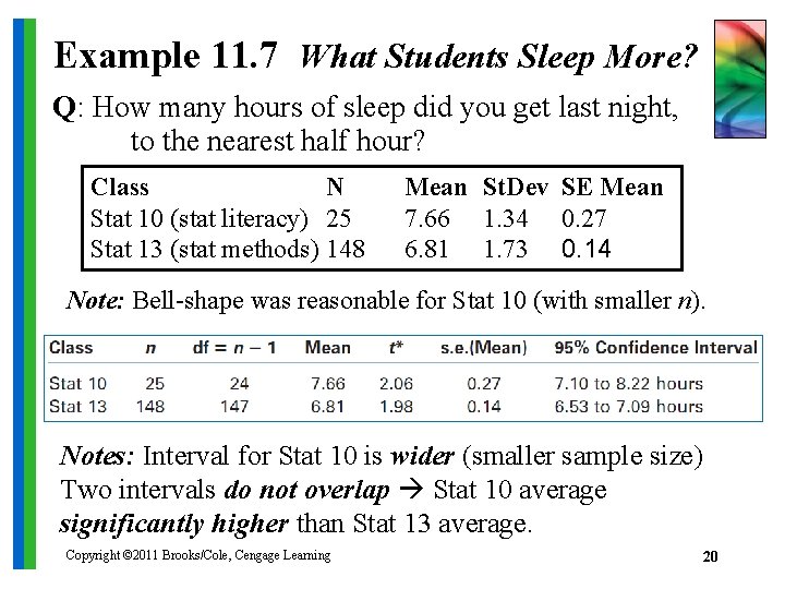
Example 11. 7 What Students Sleep More? Q: How many hours of sleep did you get last night, to the nearest half hour? Class N Stat 10 (stat literacy) 25 Stat 13 (stat methods) 148 Mean St. Dev SE Mean 7. 66 1. 34 0. 27 6. 81 1. 73 0. 14 Note: Bell-shape was reasonable for Stat 10 (with smaller n). Notes: Interval for Stat 10 is wider (smaller sample size) Two intervals do not overlap Stat 10 average significantly higher than Stat 13 average. Copyright © 2011 Brooks/Cole, Cengage Learning 20

Lesson 2: Special Case: Approximate 95% Confidence Intervals for Large Samples For sufficiently large samples, the interval Sample estimate 2 Standard error is an approximate 95% confidence interval for a population parameter. Note: The 95% confidence level describes how often the procedure provides an interval that includes the population value. For about 95% of all random samples of a specific size from a population, the confidence interval captures the population parameter. Copyright © 2011 Brooks/Cole, Cengage Learning 21

Example 11. 8 Watching TV t-Interval: 2. 09 1. 98(. 124) 2. 09 . 25 1. 84 to 2. 34 hours Approximate 95% Confidence Interval: 2. 09 2(. 124) 2. 09 . 248 1. 842 to 2. 338 hours Article: with 95% confidence, the mean is between 1. 8 and 2. 3 hours. Technically: We are 95% confident the interval from 1. 842 to 2. 338 hours is correct in that it captures the mean television viewing hours for Penn State students. Copyright © 2011 Brooks/Cole, Cengage Learning 22

11. 3 CI Module 4: CI for Population Mean of Paired Differences Data: two variables for each of the n individuals or pairs, use the difference d = x 1 – x 2 Population parameter: md = mean of the differences for the population Sample estimate: = sample mean of the differences Standard error: CI for md: Copyright © 2011 Brooks/Cole, Cengage Learning where df = n – 1 for the multiplier t* 23

11. 3 CI Module 4: CI for Population Mean of Paired Differences Data: two variables for n individuals or pairs; use the difference d = x 1 – x 2. Population parameter: md = mean of differences for the population = m 1 – m 2. Sample estimate: = sample mean of the differences Standard deviation and standard error: sd = std dev of sample of differences; Confidence interval for md: where df = n – 1 for the multiplier t*. Copyright © 2011 Brooks/Cole, Cengage Learning 24

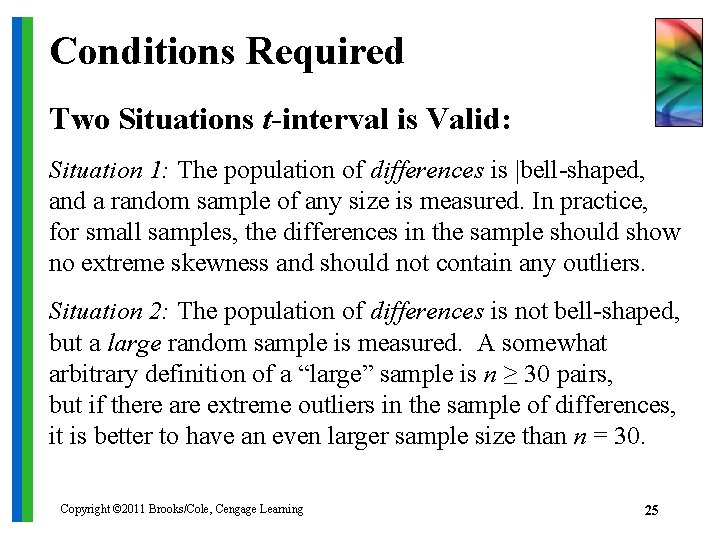
Conditions Required Two Situations t-interval is Valid: Situation 1: The population of differences is |bell-shaped, and a random sample of any size is measured. In practice, for small samples, the differences in the sample should show no extreme skewness and should not contain any outliers. Situation 2: The population of differences is not bell-shaped, but a large random sample is measured. A somewhat arbitrary definition of a “large” sample is n ≥ 30 pairs, but if there are extreme outliers in the sample of differences, it is better to have an even larger sample size than n = 30. Copyright © 2011 Brooks/Cole, Cengage Learning 25

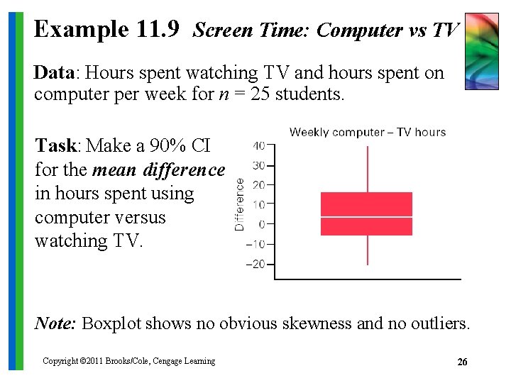
Example 11. 9 Screen Time: Computer vs TV Data: Hours spent watching TV and hours spent on computer per week for n = 25 students. Task: Make a 90% CI for the mean difference in hours spent using computer versus watching TV. Note: Boxplot shows no obvious skewness and no outliers. Copyright © 2011 Brooks/Cole, Cengage Learning 26

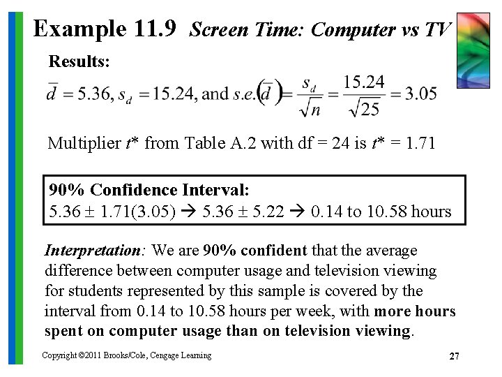
Example 11. 9 Screen Time: Computer vs TV Results: Multiplier t* from Table A. 2 with df = 24 is t* = 1. 71 90% Confidence Interval: 5. 36 1. 71(3. 05) 5. 36 5. 22 0. 14 to 10. 58 hours Interpretation: We are 90% confident that the average difference between computer usage and television viewing for students represented by this sample is covered by the interval from 0. 14 to 10. 58 hours per week, with more hours spent on computer usage than on television viewing. Copyright © 2011 Brooks/Cole, Cengage Learning 27

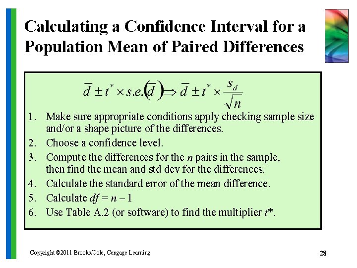
Calculating a Confidence Interval for a Population Mean of Paired Differences 1. Make sure appropriate conditions apply checking sample size and/or a shape picture of the differences. 2. Choose a confidence level. 3. Compute the differences for the n pairs in the sample, then find the mean and std dev for the differences. 4. Calculate the standard error of the mean difference. 5. Calculate df = n – 1 6. Use Table A. 2 (or software) to find the multiplier t*. Copyright © 2011 Brooks/Cole, Cengage Learning 28

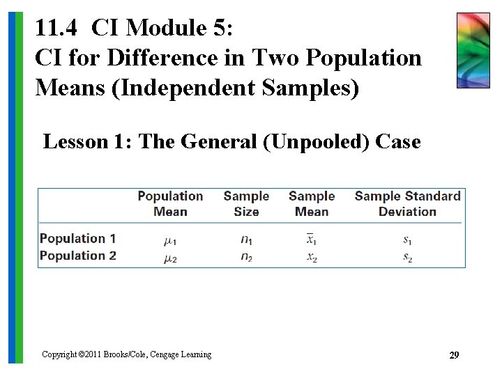
11. 4 CI Module 5: CI for Difference in Two Population Means (Independent Samples) Lesson 1: The General (Unpooled) Case Copyright © 2011 Brooks/Cole, Cengage Learning 29

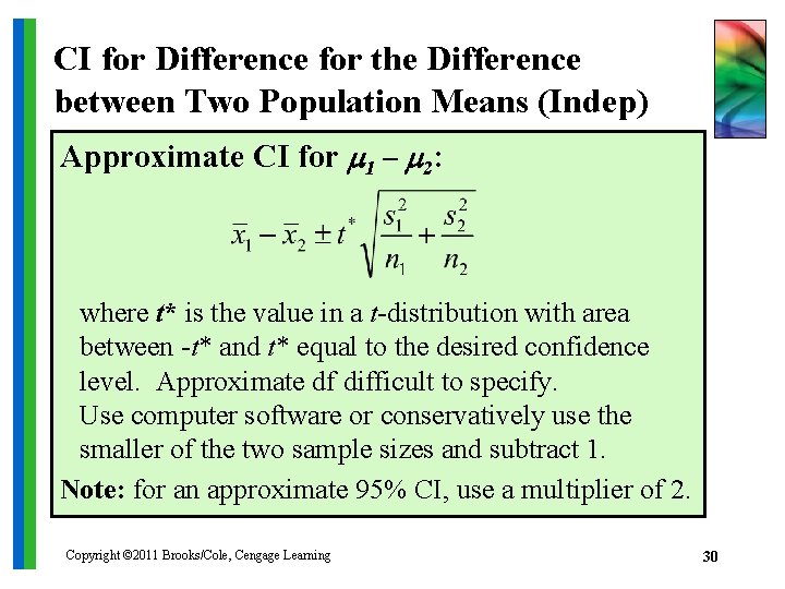
CI for Difference for the Difference between Two Population Means (Indep) Approximate CI for m 1 – m 2: where t* is the value in a t-distribution with area between -t* and t* equal to the desired confidence level. Approximate df difficult to specify. Use computer software or conservatively use the smaller of the two sample sizes and subtract 1. Note: for an approximate 95% CI, use a multiplier of 2. Copyright © 2011 Brooks/Cole, Cengage Learning 30

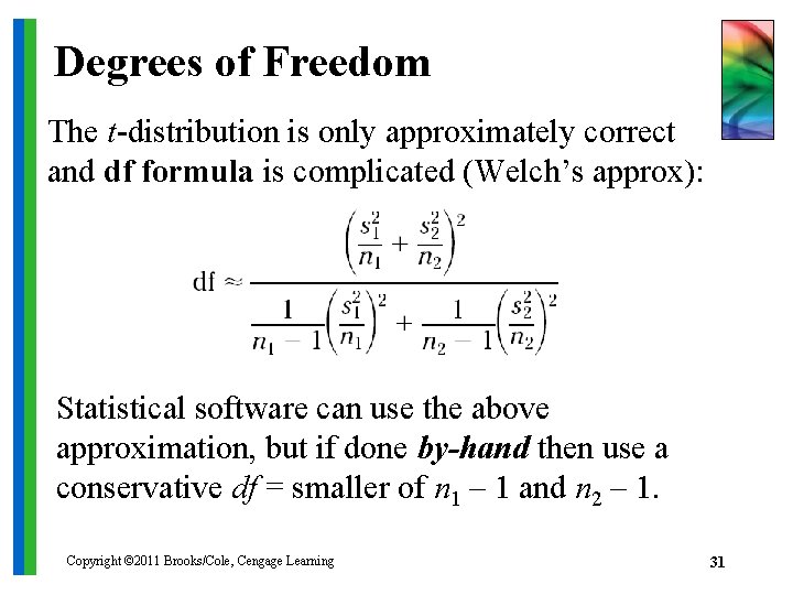
Degrees of Freedom The t-distribution is only approximately correct and df formula is complicated (Welch’s approx): Statistical software can use the above approximation, but if done by-hand then use a conservative df = smaller of n 1 – 1 and n 2 – 1. Copyright © 2011 Brooks/Cole, Cengage Learning 31

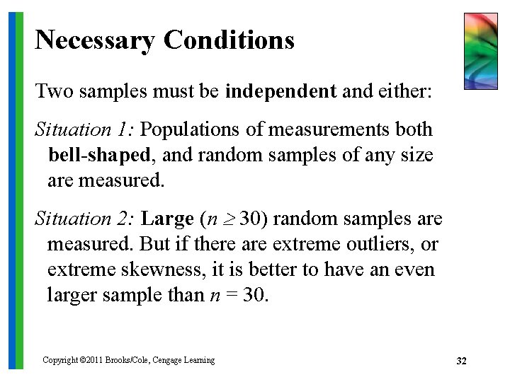
Necessary Conditions Two samples must be independent and either: Situation 1: Populations of measurements both bell-shaped, and random samples of any size are measured. Situation 2: Large (n 30) random samples are measured. But if there are extreme outliers, or extreme skewness, it is better to have an even larger sample than n = 30. Copyright © 2011 Brooks/Cole, Cengage Learning 32

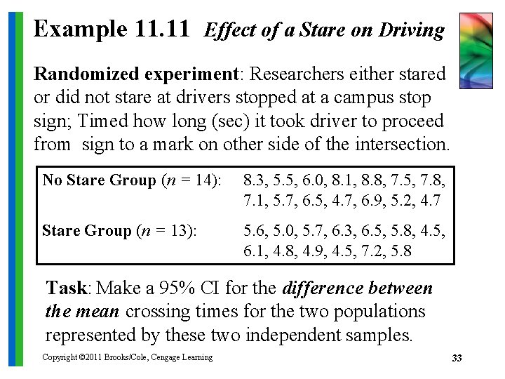
Example 11. 11 Effect of a Stare on Driving Randomized experiment: Researchers either stared or did not stare at drivers stopped at a campus stop sign; Timed how long (sec) it took driver to proceed from sign to a mark on other side of the intersection. No Stare Group (n = 14): 8. 3, 5. 5, 6. 0, 8. 1, 8. 8, 7. 5, 7. 8, 7. 1, 5. 7, 6. 5, 4. 7, 6. 9, 5. 2, 4. 7 Stare Group (n = 13): 5. 6, 5. 0, 5. 7, 6. 3, 6. 5, 5. 8, 4. 5, 6. 1, 4. 8, 4. 9, 4. 5, 7. 2, 5. 8 Task: Make a 95% CI for the difference between the mean crossing times for the two populations represented by these two independent samples. Copyright © 2011 Brooks/Cole, Cengage Learning 33

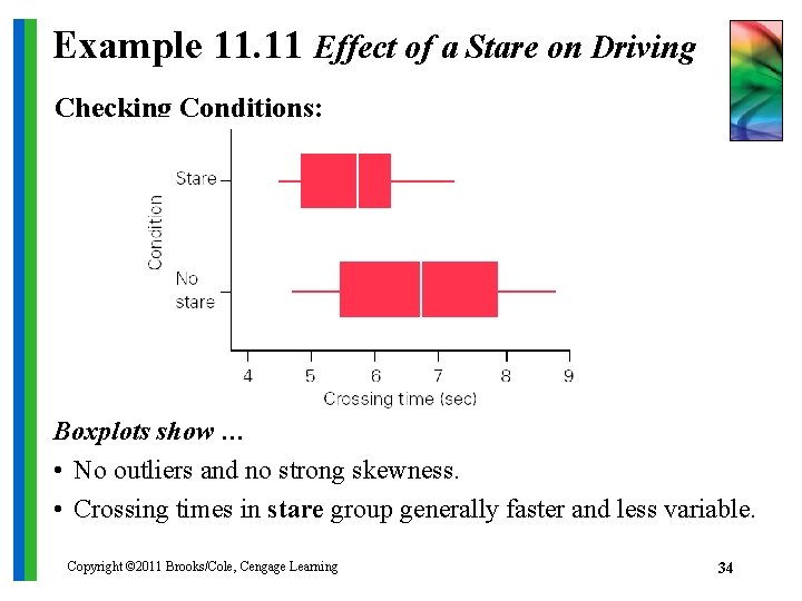
Example 11. 11 Effect of a Stare on Driving Checking Conditions: Boxplots show … • No outliers and no strong skewness. • Crossing times in stare group generally faster and less variable. Copyright © 2011 Brooks/Cole, Cengage Learning 34

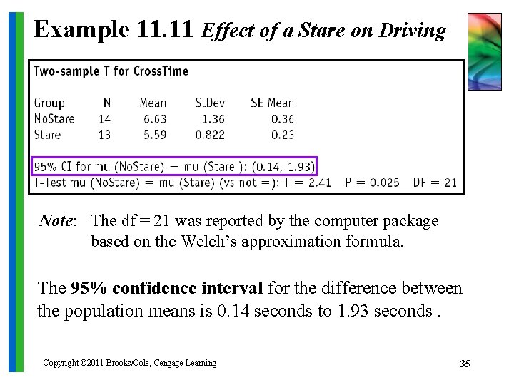
Example 11. 11 Effect of a Stare on Driving Note: The df = 21 was reported by the computer package based on the Welch’s approximation formula. The 95% confidence interval for the difference between the population means is 0. 14 seconds to 1. 93 seconds. Copyright © 2011 Brooks/Cole, Cengage Learning 35

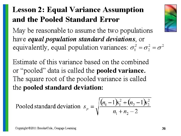
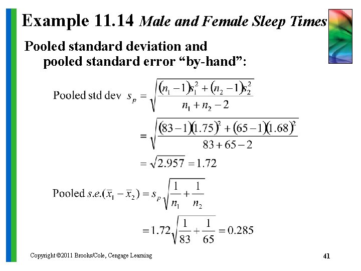
Lesson 2: Equal Variance Assumption and the Pooled Standard Error May be reasonable to assume the two populations have equal population standard deviations, or equivalently, equal population variances: Estimate of this variance based on the combined or “pooled” data is called the pooled variance. The square root of the pooled variance is called the pooled standard deviation: Copyright © 2011 Brooks/Cole, Cengage Learning 36

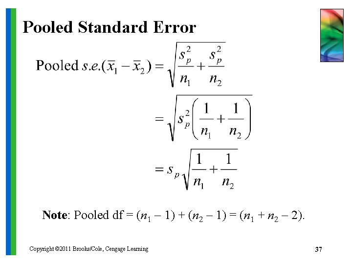
Pooled Standard Error Note: Pooled df = (n 1 – 1) + (n 2 – 1) = (n 1 + n 2 – 2). Copyright © 2011 Brooks/Cole, Cengage Learning 37

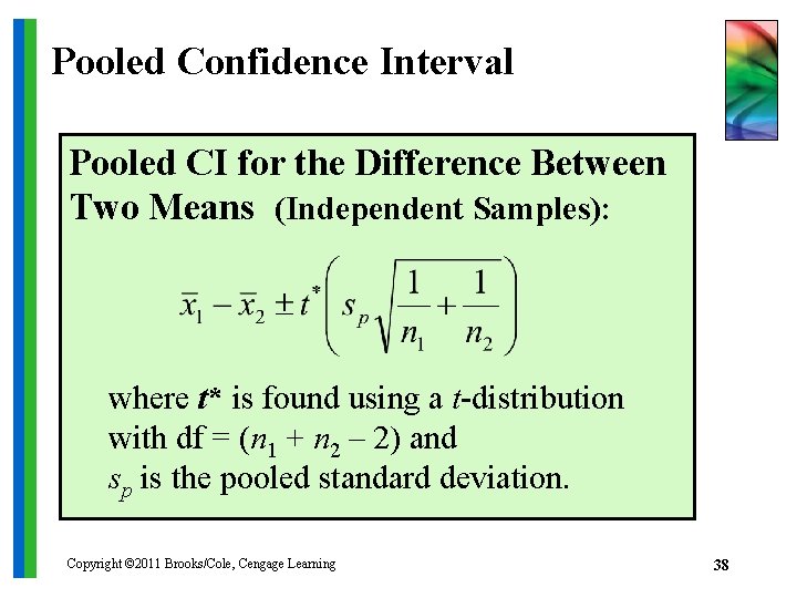
Pooled Confidence Interval Pooled CI for the Difference Between Two Means (Independent Samples): where t* is found using a t-distribution with df = (n 1 + n 2 – 2) and sp is the pooled standard deviation. Copyright © 2011 Brooks/Cole, Cengage Learning 38

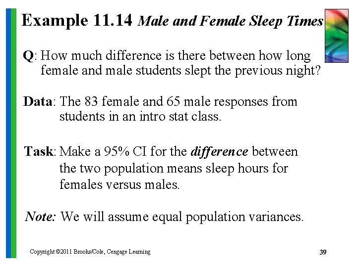
Example 11. 14 Male and Female Sleep Times Q: How much difference is there between how long female and male students slept the previous night? Data: The 83 female and 65 male responses from students in an intro stat class. Task: Make a 95% CI for the difference between the two population means sleep hours for females versus males. Note: We will assume equal population variances. Copyright © 2011 Brooks/Cole, Cengage Learning 39

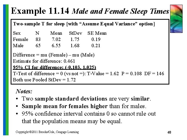
Example 11. 14 Male and Female Sleep Times Two-sample T for sleep [with “Assume Equal Variance” option] Sex Female Male N 83 65 Mean 7. 02 6. 55 St. Dev 1. 75 1. 68 SE Mean 0. 19 0. 21 Difference = mu (Female) – mu (Male) Estimate for difference: 0. 461 95% CI for difference: (-0. 103, 1. 025) T-Test of difference = 0 (vs not =): T-Value = 1. 62 P = 0. 108 DF = 146 Both use Pooled St. Dev = 1. 72 Notes: • Two sample standard deviations are very similar. • Sample mean for females higher than for males. • 95% confidence interval contains 0 so cannot rule out that the population means may be equal. Copyright © 2011 Brooks/Cole, Cengage Learning 40

Example 11. 14 Male and Female Sleep Times Pooled standard deviation and pooled standard error “by-hand”: Copyright © 2011 Brooks/Cole, Cengage Learning 41

Pooled or Unpooled? • If the larger sample size produced the larger standard deviation, the pooled procedure is acceptable because it will be conservative. • If the smaller standard deviation accompanies the larger sample size, the pooled test can be quite misleading and not recommended. • If sample sizes are equal, the pooled and unpooled standard errors are equal. Unless the sample standard deviations are quite similar, it is best to use the unpooled procedure. Copyright © 2011 Brooks/Cole, Cengage Learning 42

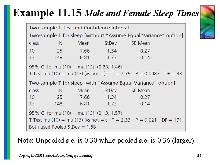
Example 11. 15 Male and Female Sleep Times Note: Unpooled s. e. is 0. 30 while pooled s. e. is 0. 36 (larger). Copyright © 2011 Brooks/Cole, Cengage Learning 43

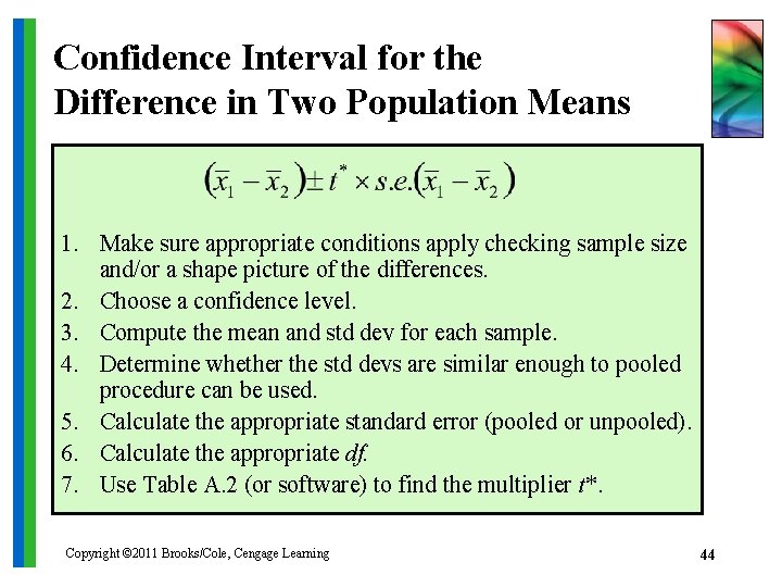
Confidence Interval for the Difference in Two Population Means 1. Make sure appropriate conditions apply checking sample size and/or a shape picture of the differences. 2. Choose a confidence level. 3. Compute the mean and std dev for each sample. 4. Determine whether the std devs are similar enough to pooled procedure can be used. 5. Calculate the appropriate standard error (pooled or unpooled). 6. Calculate the appropriate df. 7. Use Table A. 2 (or software) to find the multiplier t*. Copyright © 2011 Brooks/Cole, Cengage Learning 44