Chapter 12 Controller Design to determine controller settings

Chapter 12 Controller Design (to determine controller settings for P, PI or PID controllers) Based on Transient Response Criteria

Chapter 12 Desirable Controller Features 1. The closed-loop system must be stable. 2. The effects of disturbances are minimized, i. e. , good disturbance rejection. 3. Quick and smooth responses to the set-point changes are guaranteed, i. e. , good set-point tracking. 4. Off-set is eliminated. 5. Excessive controller action is avoided. 6. The control system is robust, i. e. , it is insensitive to changes in operating conditions and to inaccuracies in process model and/or measurements.

Chapter 12

Simplified Block Diagram

Simplified Block Diagram D(s) P(s) B(s)

Example

Chapter 12

Example 12. 1

Chapter 12

Chapter 12

Chapter 12 Alternatives for Controller Design 1. 2. 3. 4. 5. 6. Direct synthesis (DS) method Internal model control (IMC) method Controller tuning relations Frequency response techniques Computer simulation On-line tuning after the control system is installed.

Direct Synthesis

Direct Synthesis Steps 1. Specify desired closed-loop response (transfer function) 2. Assume process model 3. Solve for controller transfer function

Direct Synthesis to Achieve Perfect Control

Direct Synthesis to Achieve Finite Settling Time

Example

Example

Direct Synthesis for Time. Delayed Systems

Taylor Series Approximation

Example 1

Example 2

Pade Approximation

Example

Chapter 12 Example 12. 1 Use the DS design method to calculate PID controller settings for the process:

Chapter 12 Consider three values of the desired closed-loop time constant: . Evaluate the controllers for unit step changes in both the set point and the disturbance, assuming that Gd = G. Repeat the evaluation for two cases: a. The process model is perfect ( = G). b. The model gain is = 0. 9, instead of the actual value, K = 2. Thus, The controller settings for this example are: 3. 75 1. 88 0. 682 8. 33 4. 17 1. 51 15 3. 33

Chapter 12 Figure 12. 3 Simulation results for Example 12. 1 (a): correct model gain.

Simulation results for Example 21. 1(b): incorrect model gain.

Chapter 12

PID vs. IMC

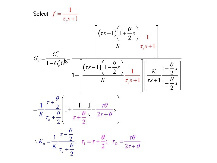
PID Controller Design Procedure Based on IMC Method –Step 1: factor process model

PID Controller Design Procedure Based on IMC Method –Step 2: derive IMC transfer function

PID Controller Design Procedure Based on IMC Method –Step 3: derive PID transfer function

Chapter 12

Example

Controller Synthesis Criteria in Time Domain Time-domain techniques can be classified into two groups: (a) Criteria based on a few points in the response (b) Criteria based on the entire response, or integral criteria

Approach (a) Based on settling time, % overshoot, rise time, decay ratio (Fig. 5. 10 can be viewed as closedloop response). Several methods based on 1/4 decay ratio have been proposed, e. g. , Cohen-Coon and Ziegler. Nichols.

Chapter 12

Chapter 12

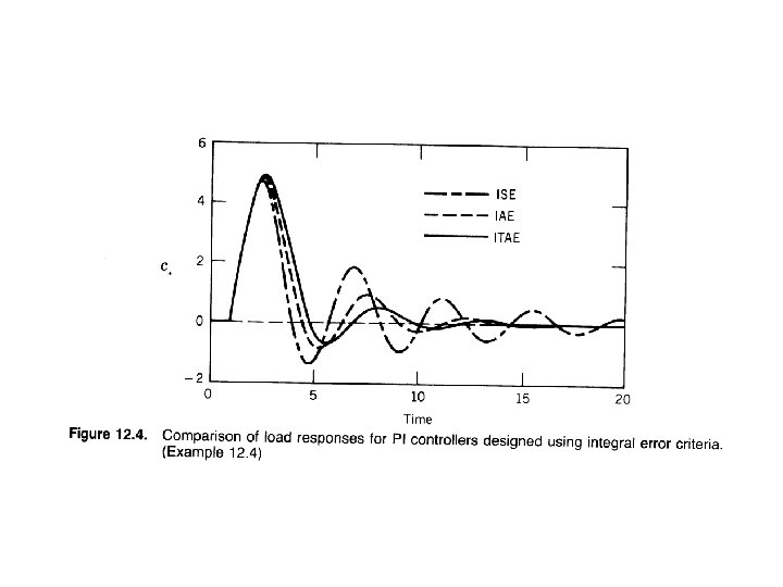
Approach (b) - Criteria • Integral of absolute value of error (IAE) • Integral of square error (ISE) • Time-weighted IAE (ITAE)

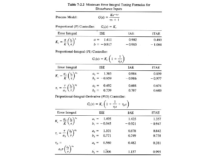
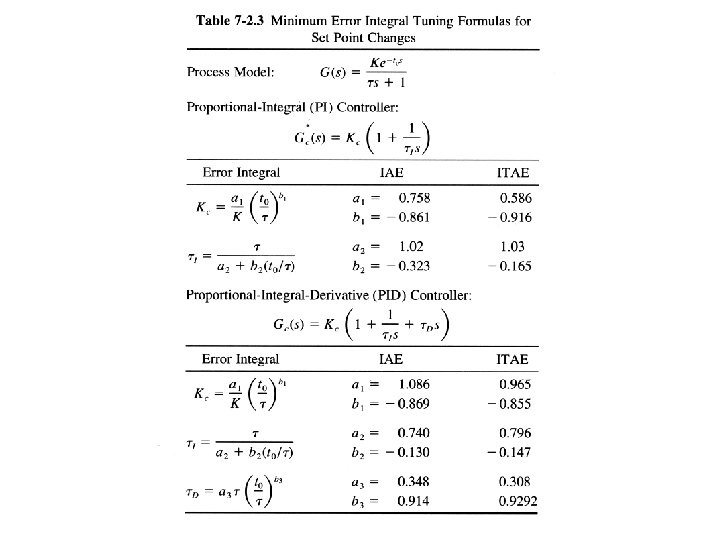
Approach (b) - Remarks Pick controller parameters to minimize integral. 1. IAE allows larger overall deviation than ISE (with smaller overshoots). 2. ISE needs longer settling time 3. ITAE weights errors occurring later more heavily Approximate optimum tuning parameters are correlated with K, , (Table 12. 3).

Chapter 12

Chapter 12

Example 1

Example 1 ITAE 0. 169 1. 85 IAE 0. 195 2. 02 ISE 0. 245 2. 44

Example 2

Chapter 12

Summary of Tuning Relationships Chapter 12 1. KC is inversely proportional to KPKVKM. 2. KC decreases as / increases. 3. I and D increase as / increases (typically D = 0. 25 I ). 4. Reduce Kc, when adding more integral action; increase Kc, when adding derivative action 5. To reduce oscillation, decrease KC and increase I.

Disadvantages of Tuning Correlations Chapter 12 1. Interactions are ignored (decreased stability limits). 2. Derivative action equipment specific. 3. First order + time delay model can be inaccurate. 4. Kp, can vary. 5. Resolution, measurement errors decrease stability margins. 6. ¼ decay ratio not conservative standard (too oscillatory).

Example 12. 4 Chapter 12 Consider a lag-dominant model with Design four PI controllers: a) IMC b) IMC 33 based on the integrator approximation in Eq. 12 - c) IMC with Skogestad’s modification (Eq. 12 -34) d) Direct Synthesis method for disturbance rejection (Chen and Seborg, 2002): The controller settings are Kc = 0. 551 and

Evaluate the four controllers by comparing their performance for unit step changes in both set point and disturbance. Assume that the model is perfect and that Gd(s) = G(s). Chapter 12 Solution The PI controller settings are: Controller Kc (a) IMC 0. 5 (b) Integrator approximation 0. 556 5 (c) Skogestad 0. 5 8 (d) DS-d 0. 551 4. 91 100

Chapter 12 Figure 12. 8. Comparison of set-point responses (top) and disturbance responses (bottom) for Example 12. 4. The responses for the Chen and Seborg and integrator approximation methods are essentially identical.

Chapter 12

On-Line Controller Tuning Chapter 12 1. Controller tuning inevitably involves a tradeoff between performance and robustness. 2. Controller settings do not have to be precisely determined. In general, a small change in a controller setting from its best value (for example, ± 10%) has little effect on closed-loop responses. 3. For most plants, it is not feasible to manually tune each controller. Tuning is usually done by a control specialist (engineer or technician) or by a plant operator. Because each person is typically responsible for 300 to 1000 control loops, it is not feasible to tune every controller. 4. Diagnostic techniques for monitoring control system performance are available.

Chapter 12 Controller Tuning and Troubleshooting Control Loops

Ziegler-Nichols Rules: Chapter 12 These well-known tuning rules were published by Z-N in 1942: controller P PI PID Kc 0. 5 KCU 0. 45 KCU 0. 6 KCU I PU/1. 2 PU/2 D PU/8 Z-N controller settings are widely considered to be an "industry standard". Z-N settings were developed to provide 1/4 decay ratio -- too oscillatory?

Modified Z-N settings for PID control Chapter 12 controller original Some overshoot No overshoot I Kc 0. 6 KCU 0. 33 KCU 0. 2 KCU PU/2 PU/3 D PU/8 PU/3 PU/2

Chapter 12

Chapter 12

Chapter 12 Figure 12. 15 Typical process reaction curves: (a) non-selfregulating process, (b) self-regulating process.

Chapter 12 Figure 12. 16 Process reaction curve for Example 12. 8.

Chapter 12 Figure 12. 17 Block diagram for Example 12. 8.

Chapter 12