Chapter 12 ChiSquare Tests and Nonparametric Tests Yandell

Chapter 12 Chi-Square Tests and Nonparametric Tests Yandell – Econ 216 Chap 12 -1

Chapter Goals After completing this chapter, you should be able to: § Perform a 2 test for the difference between two § § proportions Use a 2 test for differences in more than two proportions Perform a 2 test of independence Apply and interpret the Wilcoxon rank sum test for the difference between two medians Perform nonparametric analysis of variance using the Kruskal-Wallis rank test for one-way ANOVA Yandell – Econ 216 Chap 12 -2

Contingency Tables n n n Useful in situations involving multiple population proportions Used to classify sample observations according to two or more characteristics Also called a cross-classification table. Yandell – Econ 216 Chap 12 -3

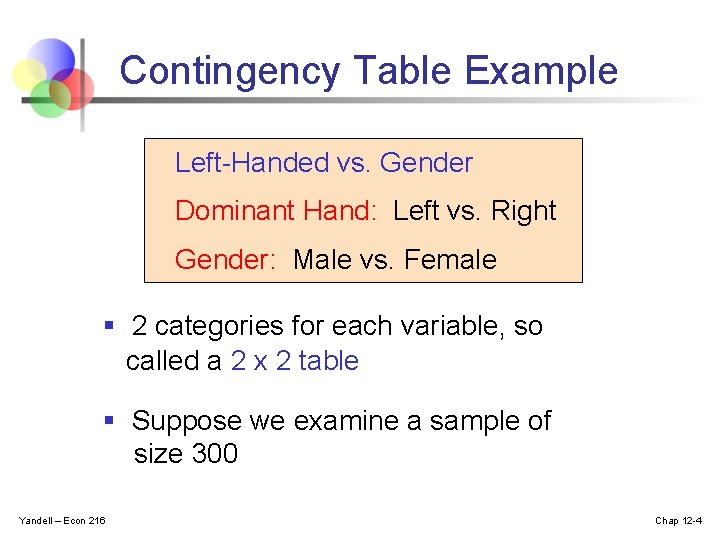
Contingency Table Example Left-Handed vs. Gender Dominant Hand: Left vs. Right Gender: Male vs. Female § 2 categories for each variable, so called a 2 x 2 table § Suppose we examine a sample of size 300 Yandell – Econ 216 Chap 12 -4

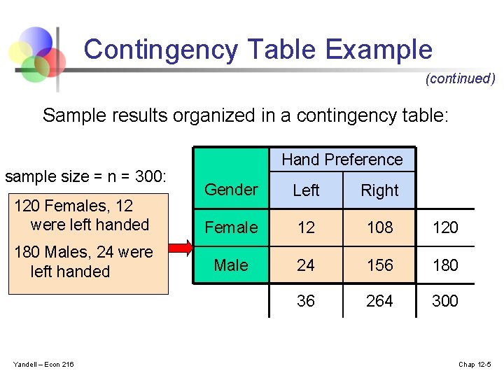
Contingency Table Example (continued) Sample results organized in a contingency table: sample size = n = 300: 120 Females, 12 were left handed 180 Males, 24 were left handed Yandell – Econ 216 Hand Preference Gender Left Right Female 12 108 120 Male 24 156 180 36 264 300 Chap 12 -5

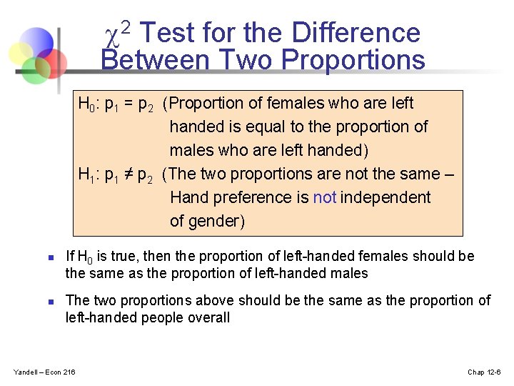
2 Test for the Difference Between Two Proportions H 0: p 1 = p 2 (Proportion of females who are left handed is equal to the proportion of males who are left handed) H 1: p 1 ≠ p 2 (The two proportions are not the same – Hand preference is not independent of gender) n n If H 0 is true, then the proportion of left-handed females should be the same as the proportion of left-handed males The two proportions above should be the same as the proportion of left-handed people overall Yandell – Econ 216 Chap 12 -6

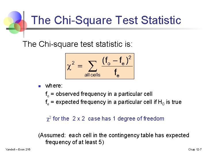
The Chi-Square Test Statistic The Chi-square test statistic is: n where: fo = observed frequency in a particular cell fe = expected frequency in a particular cell if H 0 is true 2 for the 2 x 2 case has 1 degree of freedom (Assumed: each cell in the contingency table has expected frequency of at least 5) Yandell – Econ 216 Chap 12 -7

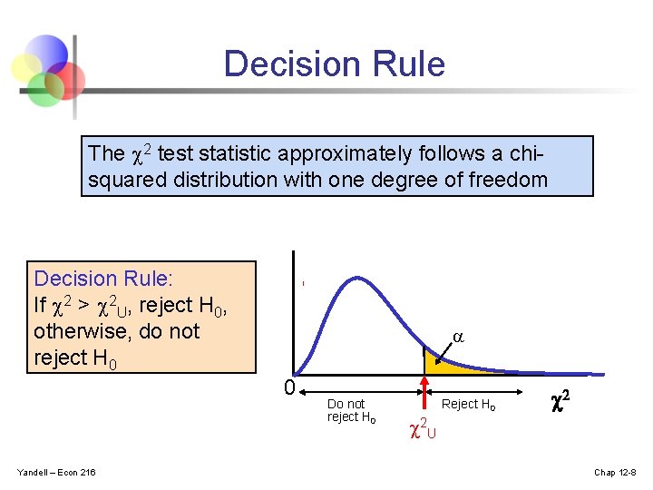
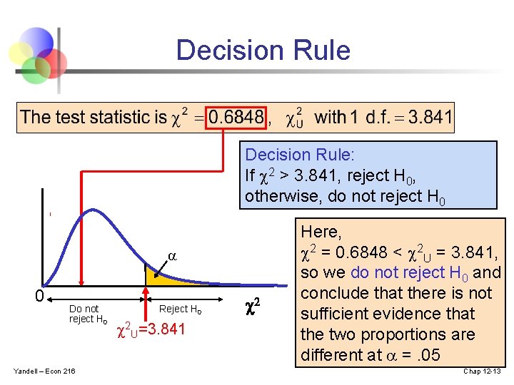
Decision Rule The 2 test statistic approximately follows a chisquared distribution with one degree of freedom Decision Rule: If 2 > 2 U, reject H 0, otherwise, do not reject H 0 0 Yandell – Econ 216 Do not reject H 0 Reject H 0 2 2 U Chap 12 -8

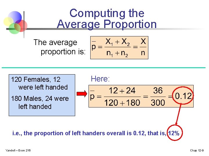
Computing the Average Proportion The average proportion is: 120 Females, 12 were left handed Here: 180 Males, 24 were left handed i. e. , the proportion of left handers overall is 0. 12, that is, 12% Yandell – Econ 216 Chap 12 -9

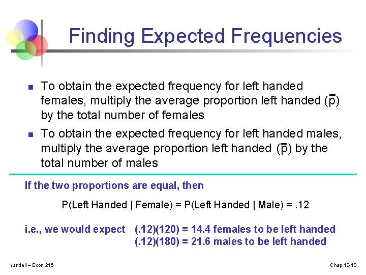
Finding Expected Frequencies n n To obtain the expected frequency for left handed females, multiply the average proportion left handed (p) by the total number of females To obtain the expected frequency for left handed males, multiply the average proportion left handed (p) by the total number of males If the two proportions are equal, then P(Left Handed | Female) = P(Left Handed | Male) =. 12 i. e. , we would expect (. 12)(120) = 14. 4 females to be left handed (. 12)(180) = 21. 6 males to be left handed Yandell – Econ 216 Chap 12 -10

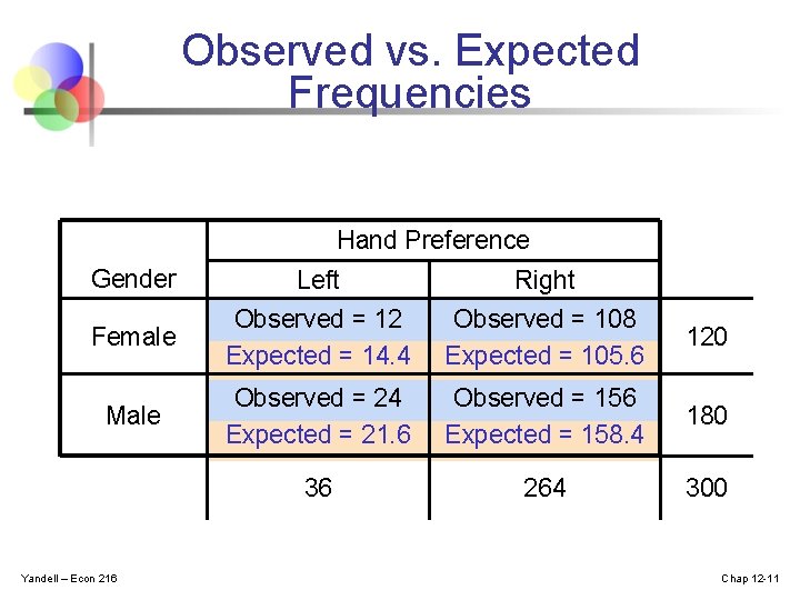
Observed vs. Expected Frequencies Hand Preference Gender Left Right Female Observed = 12 Expected = 14. 4 Observed = 108 Expected = 105. 6 120 Male Observed = 24 Expected = 21. 6 Observed = 156 Expected = 158. 4 180 36 264 300 Yandell – Econ 216 Chap 12 -11

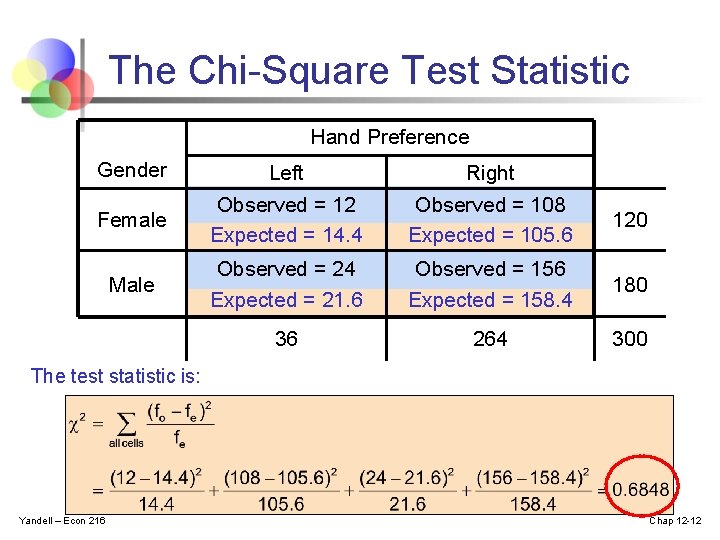
The Chi-Square Test Statistic Hand Preference Gender Left Right Female Observed = 12 Expected = 14. 4 Observed = 108 Expected = 105. 6 120 Male Observed = 24 Expected = 21. 6 Observed = 156 Expected = 158. 4 180 36 264 300 The test statistic is: Yandell – Econ 216 Chap 12 -12

Decision Rule: If 2 > 3. 841, reject H 0, otherwise, do not reject H 0 0 Do not reject H 0 Yandell – Econ 216 Reject H 0 2 U=3. 841 2 Here, 2 = 0. 6848 < 2 U = 3. 841, so we do not reject H 0 and conclude that there is not sufficient evidence that the two proportions are different at =. 05 Chap 12 -13

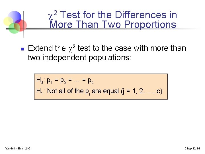
2 Test for the Differences in More Than Two Proportions n Extend the 2 test to the case with more than two independent populations: H 0: p 1 = p 2 = … = p c H 1: Not all of the pj are equal (j = 1, 2, …, c) Yandell – Econ 216 Chap 12 -14

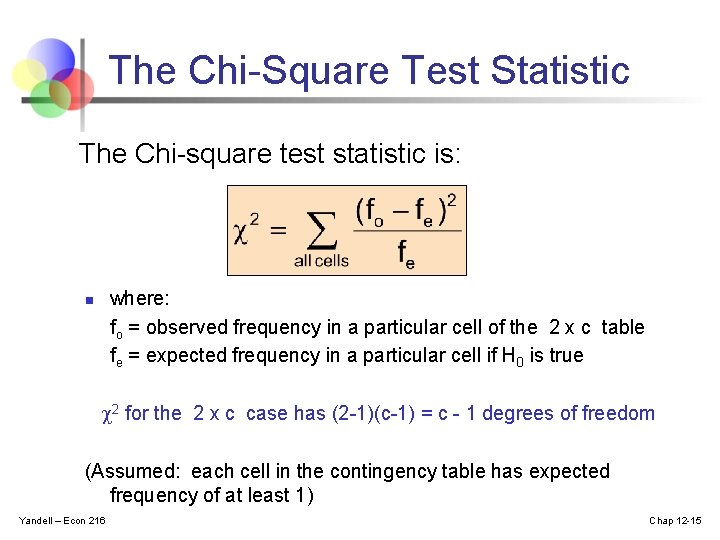
The Chi-Square Test Statistic The Chi-square test statistic is: where: fo = observed frequency in a particular cell of the 2 x c table fe = expected frequency in a particular cell if H 0 is true n 2 for the 2 x c case has (2 -1)(c-1) = c - 1 degrees of freedom (Assumed: each cell in the contingency table has expected frequency of at least 1) Yandell – Econ 216 Chap 12 -15

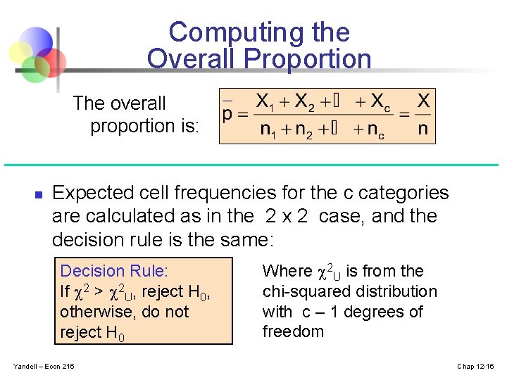
Computing the Overall Proportion The overall proportion is: n Expected cell frequencies for the c categories are calculated as in the 2 x 2 case, and the decision rule is the same: Decision Rule: If 2 > 2 U, reject H 0, otherwise, do not reject H 0 Yandell – Econ 216 Where 2 U is from the chi-squared distribution with c – 1 degrees of freedom Chap 12 -16

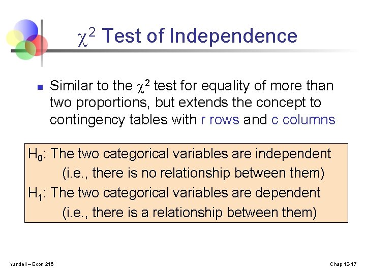
2 Test of Independence n Similar to the 2 test for equality of more than two proportions, but extends the concept to contingency tables with r rows and c columns H 0: The two categorical variables are independent (i. e. , there is no relationship between them) H 1: The two categorical variables are dependent (i. e. , there is a relationship between them) Yandell – Econ 216 Chap 12 -17

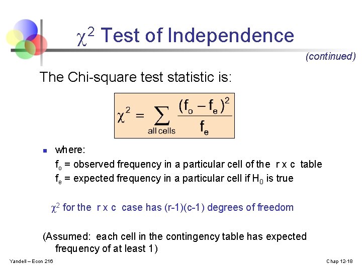
2 Test of Independence (continued) The Chi-square test statistic is: where: fo = observed frequency in a particular cell of the r x c table fe = expected frequency in a particular cell if H 0 is true n 2 for the r x c case has (r-1)(c-1) degrees of freedom (Assumed: each cell in the contingency table has expected frequency of at least 1) Yandell – Econ 216 Chap 12 -18

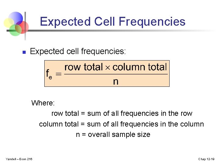
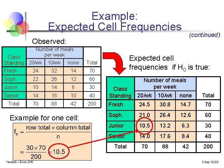
Expected Cell Frequencies n Expected cell frequencies: Where: row total = sum of all frequencies in the row column total = sum of all frequencies in the column n = overall sample size Yandell – Econ 216 Chap 12 -19

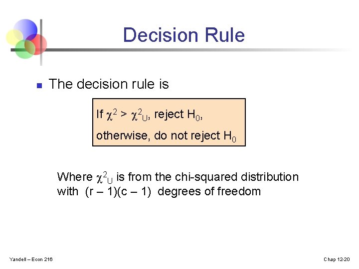
Decision Rule n The decision rule is If 2 > 2 U, reject H 0, otherwise, do not reject H 0 Where 2 U is from the chi-squared distribution with (r – 1)(c – 1) degrees of freedom Yandell – Econ 216 Chap 12 -20

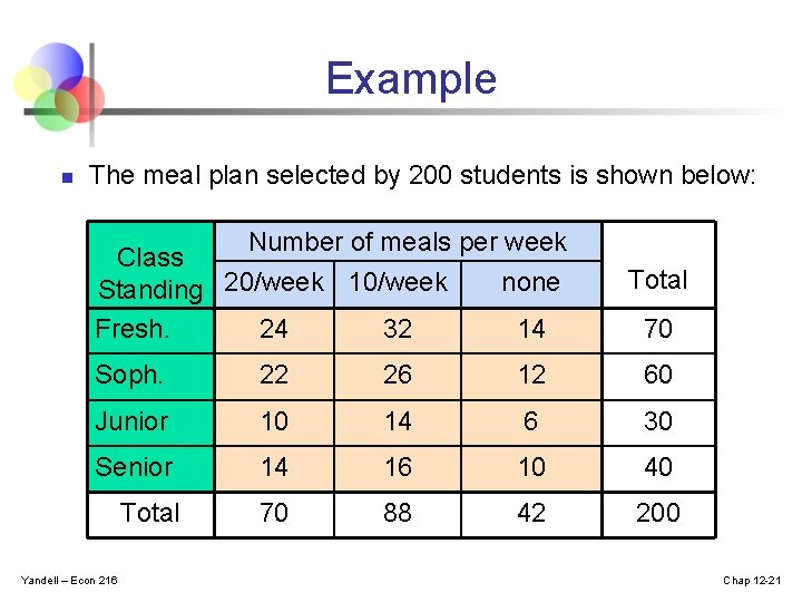
Example n The meal plan selected by 200 students is shown below: Number of meals per week Class none Standing 20/week 10/week Fresh. 24 32 14 Total 70 Soph. 22 26 12 60 Junior 10 14 6 30 Senior 14 16 10 40 Total 70 88 42 200 Yandell – Econ 216 Chap 12 -21

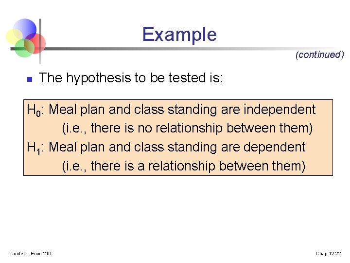
Example (continued) n The hypothesis to be tested is: H 0: Meal plan and class standing are independent (i. e. , there is no relationship between them) H 1: Meal plan and class standing are dependent (i. e. , there is a relationship between them) Yandell – Econ 216 Chap 12 -22

Example: Expected Cell Frequencies (continued) Observed: Class Standing Number of meals per week Expected cell frequencies if H 0 is true: 20/wk 10/wk none Total Fresh. 24 32 14 70 Soph. 22 26 12 60 Junior 10 14 6 30 Senior 14 16 10 40 Class Standing Total 70 88 42 200 Example for one cell: 20/wk 10/wk none Total Fresh. 24. 5 30. 8 14. 7 70 Soph. 21. 0 26. 4 12. 6 60 Junior 10. 5 13. 2 6. 3 30 Senior 14. 0 17. 6 8. 4 40 70 88 42 200 Total Yandell – Econ 216 Number of meals per week Chap 12 -23

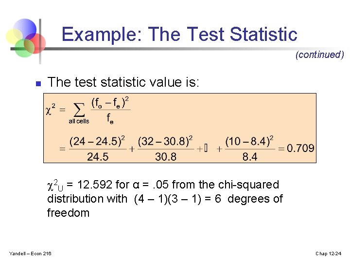
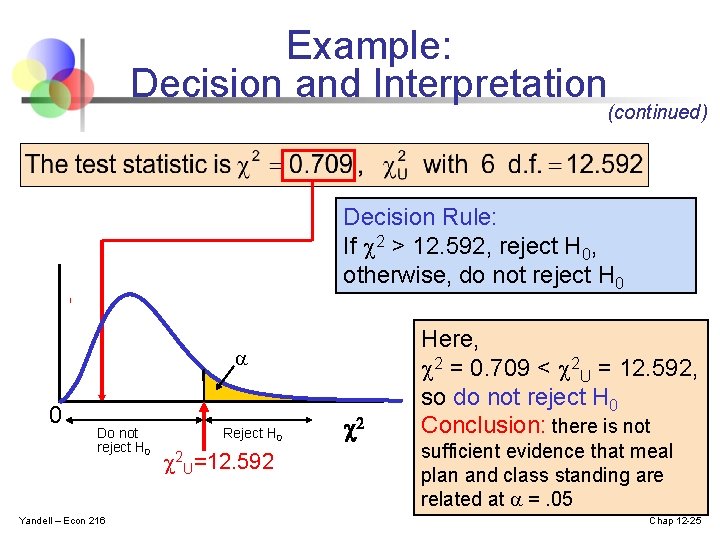
Example: The Test Statistic (continued) n The test statistic value is: 2 U = 12. 592 for α =. 05 from the chi-squared distribution with (4 – 1)(3 – 1) = 6 degrees of freedom Yandell – Econ 216 Chap 12 -24

Example: Decision and Interpretation (continued) Decision Rule: If 2 > 12. 592, reject H 0, otherwise, do not reject H 0 0 Do not reject H 0 Yandell – Econ 216 Reject H 0 2 U=12. 592 2 Here, 2 = 0. 709 < 2 U = 12. 592, so do not reject H 0 Conclusion: there is not sufficient evidence that meal plan and class standing are related at =. 05 Chap 12 -25

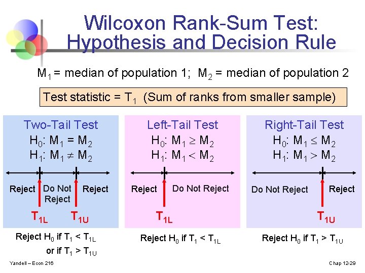
Wilcoxon Rank-Sum Test for Differences in 2 Medians n Test two independent population medians n Populations need not be normally distributed n Distribution free procedure n Used when only rank data are available n Must use normal approximation if either of the sample sizes is larger than 10 Yandell – Econ 216 Chap 12 -26

Wilcoxon Rank-Sum Test: Small Samples n n Can use when both n 1 , n 2 ≤ 10 Assign ranks to the combined n 1 + n 2 sample observations n n n If unequal sample sizes, let n 1 refer to smaller-sized sample Smallest value rank = 1, largest value rank = n 1 + n 2 Assign average rank for ties n Sum the ranks for each sample: T 1 and T 2 n Obtain test statistic, T 1 (from smaller sample) Yandell – Econ 216 Chap 12 -27

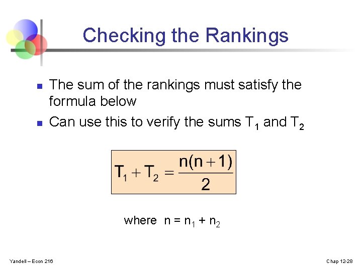
Checking the Rankings n n The sum of the rankings must satisfy the formula below Can use this to verify the sums T 1 and T 2 where n = n 1 + n 2 Yandell – Econ 216 Chap 12 -28

Wilcoxon Rank-Sum Test: Hypothesis and Decision Rule M 1 = median of population 1; M 2 = median of population 2 Test statistic = T 1 (Sum of ranks from smaller sample) Two-Tail Test H 0: M 1 = M 2 H 1: M 1 ¹ M 2 Reject Do Not Reject T 1 L Reject T 1 U Reject H 0 if T 1 < T 1 L Left-Tail Test H 0: M 1 ³ M 2 H 1: M 1 < M 2 Reject Do Not Reject T 1 L Reject H 0 if T 1 < T 1 L Right-Tail Test H 0: M 1 £ M 2 H 1: M 1 > M 2 Do Not Reject T 1 U Reject H 0 if T 1 > T 1 U or if T 1 > T 1 U Yandell – Econ 216 Chap 12 -29

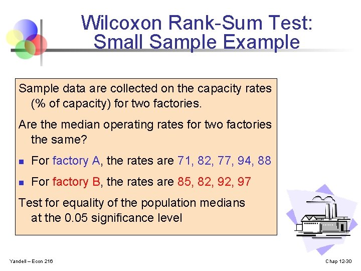
Wilcoxon Rank-Sum Test: Small Sample Example Sample data are collected on the capacity rates (% of capacity) for two factories. Are the median operating rates for two factories the same? n For factory A, the rates are 71, 82, 77, 94, 88 n For factory B, the rates are 85, 82, 97 Test for equality of the population medians at the 0. 05 significance level Yandell – Econ 216 Chap 12 -30

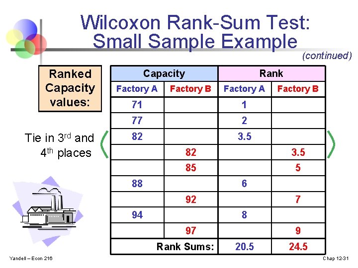
Wilcoxon Rank-Sum Test: Small Sample Example (continued) Ranked Capacity values: Tie in 3 rd and 4 th places Capacity Factory A Rank Factory B Factory A 71 1 77 2 82 3. 5 85 5 88 6 92 94 7 8 97 Rank Sums: Yandell – Econ 216 Factory B 9 20. 5 24. 5 Chap 12 -31

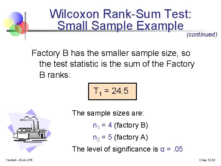
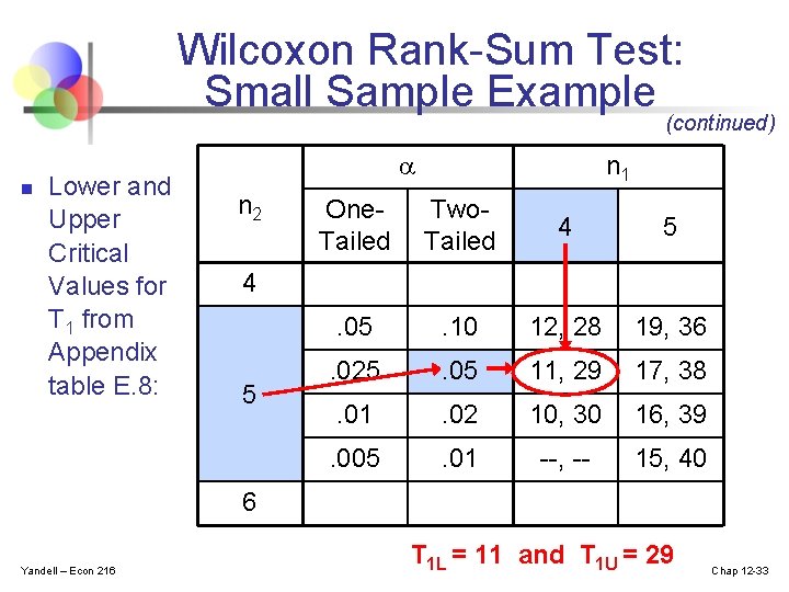
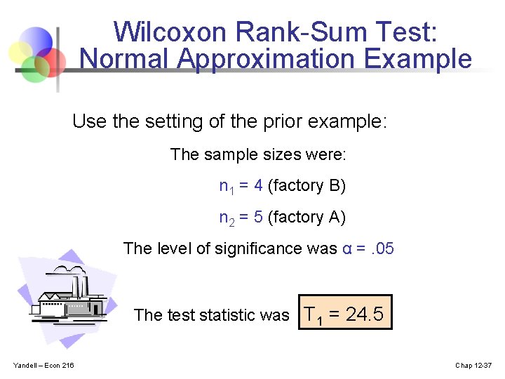
Wilcoxon Rank-Sum Test: Small Sample Example (continued) Factory B has the smaller sample size, so the test statistic is the sum of the Factory B ranks: T 1 = 24. 5 The sample sizes are: n 1 = 4 (factory B) n 2 = 5 (factory A) The level of significance is α =. 05 Yandell – Econ 216 Chap 12 -32

Wilcoxon Rank-Sum Test: Small Sample Example (continued) n Lower and Upper Critical Values for T 1 from Appendix table E. 8: n 2 n 1 One. Tailed Two. Tailed 4 5 . 05 . 10 12, 28 19, 36 . 025 . 05 11, 29 17, 38 . 01 . 02 10, 30 16, 39 . 005 . 01 --, -- 15, 40 4 5 6 Yandell – Econ 216 T 1 L = 11 and T 1 U = 29 Chap 12 -33

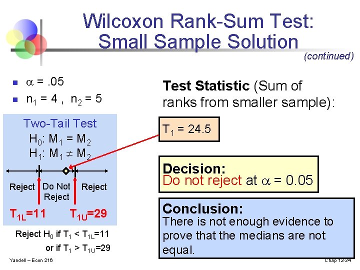
Wilcoxon Rank-Sum Test: Small Sample Solution (continued) n n =. 05 n 1 = 4 , n 2 = 5 Test Statistic (Sum of ranks from smaller sample): Two-Tail Test H 0: M 1 = M 2 H 1: M 1 ¹ M 2 T 1 = 24. 5 Reject Do Not Reject T 1 L=11 Reject T 1 U=29 Reject H 0 if T 1 < T 1 L=11 or if T 1 > T 1 U=29 Yandell – Econ 216 Decision: Do not reject at = 0. 05 Conclusion: There is not enough evidence to prove that the medians are not equal. Chap 12 -34

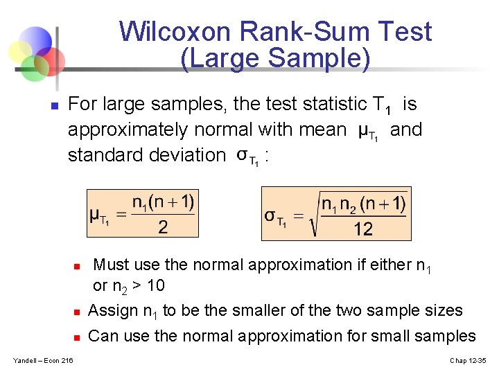
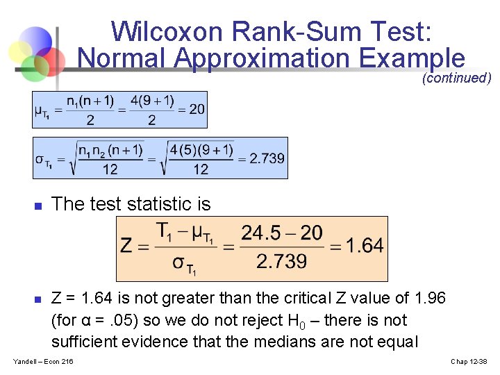
Wilcoxon Rank-Sum Test (Large Sample) n For large samples, the test statistic T 1 is approximately normal with mean and standard deviation : n Must use the normal approximation if either n 1 or n 2 > 10 Assign n 1 to be the smaller of the two sample sizes n Can use the normal approximation for small samples n Yandell – Econ 216 Chap 12 -35

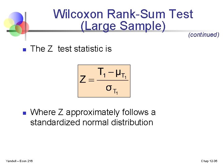
Wilcoxon Rank-Sum Test (Large Sample) (continued) n n The Z test statistic is Where Z approximately follows a standardized normal distribution Yandell – Econ 216 Chap 12 -36

Wilcoxon Rank-Sum Test: Normal Approximation Example Use the setting of the prior example: The sample sizes were: n 1 = 4 (factory B) n 2 = 5 (factory A) The level of significance was α =. 05 The test statistic was T 1 = 24. 5 Yandell – Econ 216 Chap 12 -37

Wilcoxon Rank-Sum Test: Normal Approximation Example (continued) n n The test statistic is Z = 1. 64 is not greater than the critical Z value of 1. 96 (for α =. 05) so we do not reject H 0 – there is not sufficient evidence that the medians are not equal Yandell – Econ 216 Chap 12 -38

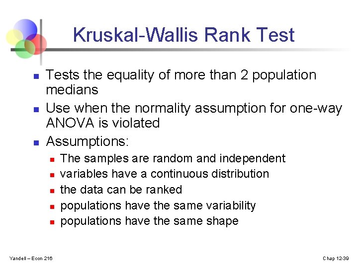
Kruskal-Wallis Rank Test n n n Tests the equality of more than 2 population medians Use when the normality assumption for one-way ANOVA is violated Assumptions: n n n Yandell – Econ 216 The samples are random and independent variables have a continuous distribution the data can be ranked populations have the same variability populations have the same shape Chap 12 -39

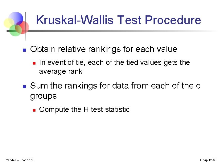
Kruskal-Wallis Test Procedure n Obtain relative rankings for each value n n In event of tie, each of the tied values gets the average rank Sum the rankings for data from each of the c groups n Yandell – Econ 216 Compute the H test statistic Chap 12 -40

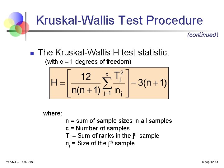
Kruskal-Wallis Test Procedure (continued) n The Kruskal-Wallis H test statistic: (with c – 1 degrees of freedom) where: n = sum of sample sizes in all samples c = Number of samples Tj = Sum of ranks in the jth sample nj = Size of the jth sample Yandell – Econ 216 Chap 12 -41

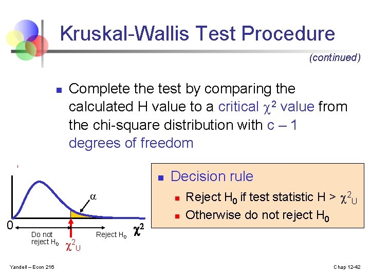
Kruskal-Wallis Test Procedure (continued) n Complete the test by comparing the calculated H value to a critical 2 value from the chi-square distribution with c – 1 degrees of freedom n 0 Do not reject H 0 Yandell – Econ 216 2 U Reject H 0 Decision rule n 2 n Reject H 0 if test statistic H > 2 U Otherwise do not reject H 0 Chap 12 -42

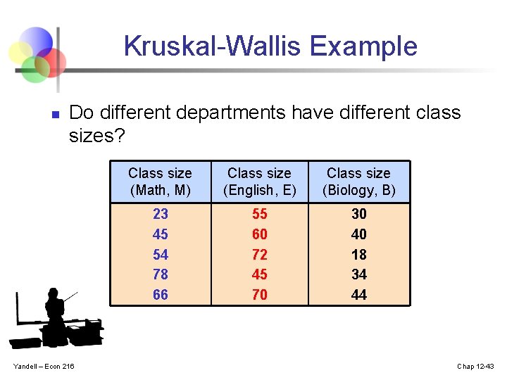
Kruskal-Wallis Example n Do different departments have different class sizes? Yandell – Econ 216 Class size (Math, M) Class size (English, E) Class size (Biology, B) 23 45 54 78 66 55 60 72 45 70 30 40 18 34 44 Chap 12 -43

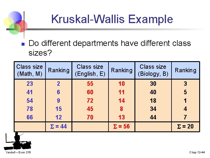
Kruskal-Wallis Example n Do different departments have different class sizes? Class size Ranking (Math, M) (English, E) (Biology, B) 23 41 54 78 66 2 6 9 15 12 = 44 Yandell – Econ 216 55 60 72 45 70 10 11 14 8 13 = 56 30 40 18 34 44 Ranking 3 5 1 4 7 = 20 Chap 12 -44

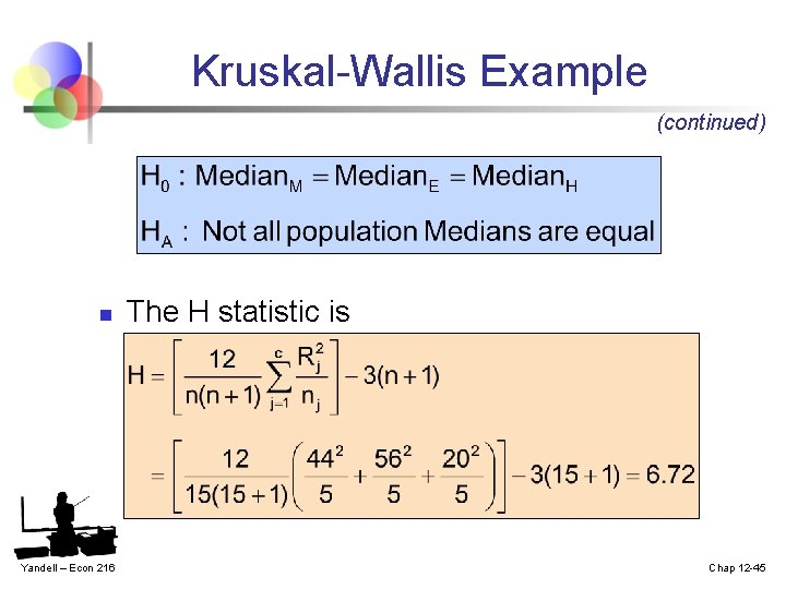
Kruskal-Wallis Example (continued) n Yandell – Econ 216 The H statistic is Chap 12 -45

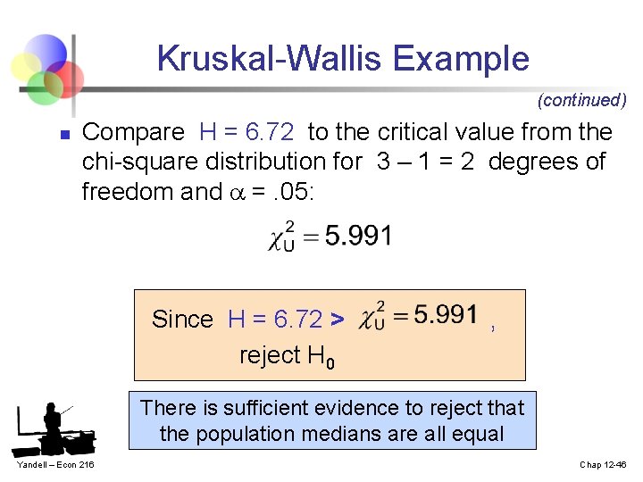
Kruskal-Wallis Example (continued) n Compare H = 6. 72 to the critical value from the chi-square distribution for 3 – 1 = 2 degrees of freedom and =. 05: Since H = 6. 72 > reject H 0 , There is sufficient evidence to reject that the population medians are all equal Yandell – Econ 216 Chap 12 -46

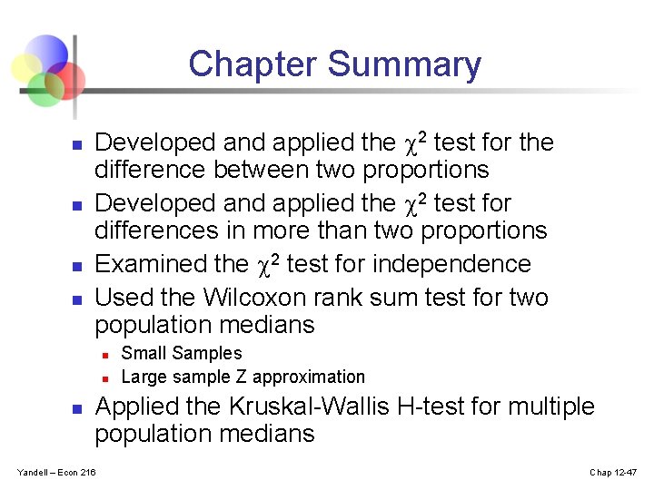
Chapter Summary n n Developed and applied the 2 test for the difference between two proportions Developed and applied the 2 test for differences in more than two proportions Examined the 2 test for independence Used the Wilcoxon rank sum test for two population medians n n n Small Samples Large sample Z approximation Applied the Kruskal-Wallis H-test for multiple population medians Yandell – Econ 216 Chap 12 -47