CHAPTER 12 ANALYSIS OF VARIANCE Presented by Hessa

CHAPTER 12 ANALYSIS OF VARIANCE Presented by: Hessa Alangeri Sara Aldaej

Outlines • One-Way ANOVA • Hypothesis testing • Comparisons of groups 12. 1 - 2

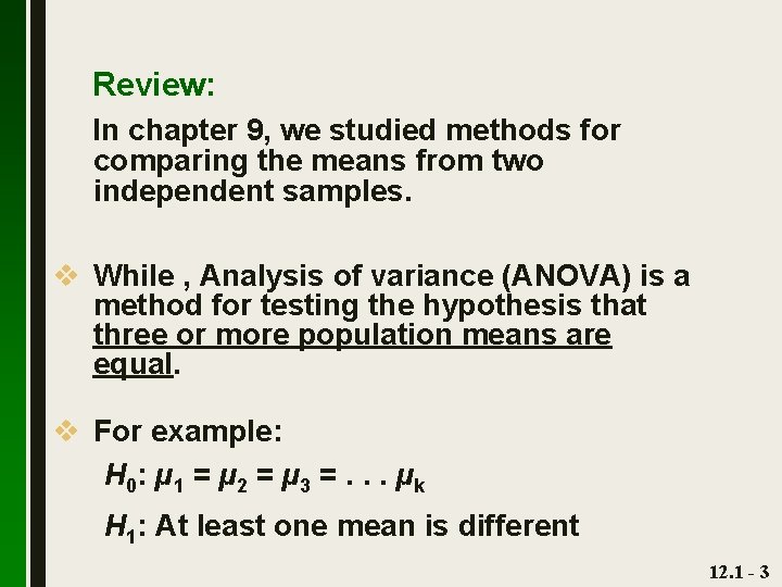
Review: In chapter 9, we studied methods for comparing the means from two independent samples. v While , Analysis of variance (ANOVA) is a method for testing the hypothesis that three or more population means are equal. v For example: H 0: µ 1 = µ 2 = µ 3 =. . . µ k H 1: At least one mean is different 12. 1 - 3

Key Concept This section introduces the method of one-way analysis of variance, which is used for tests of hypotheses that three or more population means are all equal. 12. 1 - 4

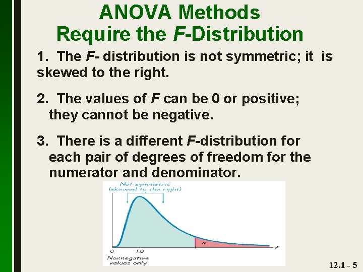
ANOVA Methods Require the F-Distribution 1. The F- distribution is not symmetric; it is skewed to the right. 2. The values of F can be 0 or positive; they cannot be negative. 3. There is a different F-distribution for each pair of degrees of freedom for the numerator and denominator. 12. 1 - 5

PART 1: BASICS OF ONE-WAY ANALYSIS OF VARIANCE 12. 1 - 6

Definition One-way analysis of variance (ANOVA) is a method of testing the equality of three or more population means by analyzing sample variances. One-way analysis of variance is used with data categorized with one treatment (or factor), which is a characteristic that allows us to distinguish the different populations from one another. 12. 1 - 7

One-Way ANOVA Requirements 1. The populations have approximately normal. 2. The populations have the same variance 2 (or standard deviation ). 3. The samples are simple random samples. 4. The samples are independent of each other. 5. The different samples are from populations that are categorized in only one way. 12. 1 - 8

Procedure for testing H 0: µ 1 = µ 2 = µ 3 =. . . 1. Use technology to obtain results. 2. Identify the P-value from the display. 3. Form a conclusion based on these criteria: • Reject, • Fail to reject 12. 1 - 9

Procedure for testing H 0: µ 1 = µ 2 = µ 3 =. . . If the P-value , reject the null hypothesis of equal means and conclude that at least one of the population means is different from the others. If the P-value > , fail to reject the null hypothesis of equal means. 12. 1 - 10

One-Way ANOVA An Approach to Understanding ANOVA 1. Understand that a small P-value (such as 0. 05 or less) leads to rejection of the null hypothesis of equal means. With a large P-value (such as greater than 0. 05), fail to reject the null hypothesis of equal means. 2. Develop an understanding of the underlying rationale by studying the examples in this section. 12. 1 - 11

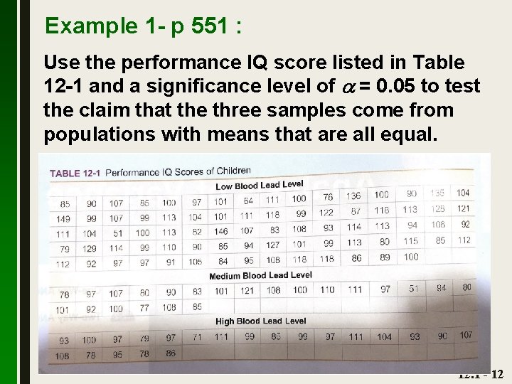
Example 1 - p 551 : Use the performance IQ score listed in Table 12 -1 and a significance level of = 0. 05 to test the claim that the three samples come from populations with means that are all equal. 12. 1 - 12

Example: Requirements are satisfied: distributions are approximately normal (normal quantile plots); population variances appear to be about the same; simple random samples; independent samples, not matched; categorized according to a single factor of size H 0: 1 = 2 = 3 H 1: At least one of the means is different from the others significance level is = 0. 05 12. 1 - 13

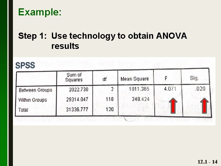
Example: Step 1: Use technology to obtain ANOVA results 12. 1 - 14

Example: Step 2: in addition to the test statistic of F = 4. 0711, Display shows P-value = 0. 020 when rounded Step 3: Because the P-value of 0. 020 is less than the significance level of = 0. 05, we reject the null hypothesis of equal means. Ø There is sufficient evidence to warrant rejection of the claim that the three samples come from populations with means that are all equal. 12. 1 - 15

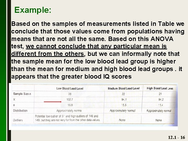
Example: Based on the samples of measurements listed in Table we conclude that those values come from populations having means that are not all the same. Based on this ANOVA test, we cannot conclude that any particular mean is different from the others, but we can informally note that the sample mean for the low blood lead group is higher than the mean for medium and high blood lead groups. it appears that the greater blood IQ scores 12. 1 - 16

Caution There are several other tests that can be used to identify the specific means that are different, and some of them are discussed in Part 2 of this section. 12. 1 - 17

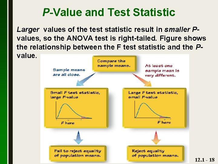
P-Value and Test Statistic Larger values of the test statistic result in smaller Pvalues, so the ANOVA test is right-tailed. Figure shows the relationship between the F test statistic and the Pvalue. 12. 1 - 18

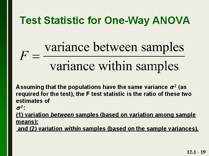
Test Statistic for One-Way ANOVA Assuming that the populations have the same variance 2 (as required for the test), the F test statistic is the ratio of these two estimates of 2: (1) variation between samples (based on variation among sample means); and (2) variation within samples (based on the sample variances). 12. 1 - 19

Caution When testing for equality of three or more populations, use analysis of variance. Do not use multiple hypothesis tests with two samples at a time. 12. 1 - 20

PART 2: CALCULATIONS AND IDENTIFYING MEANS THAT ARE DIFFERENT 12. 1 - 21

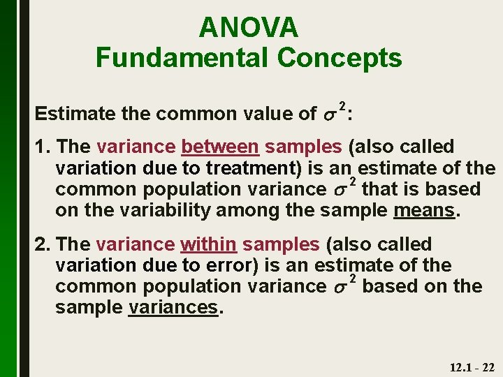
ANOVA Fundamental Concepts 2 Estimate the common value of : 1. The variance between samples (also called variation due to treatment) is an estimate of the common population variance 2 that is based on the variability among the sample means. 2. The variance within samples (also called variation due to error) is an estimate of the common population variance 2 based on the sample variances. 12. 1 - 22

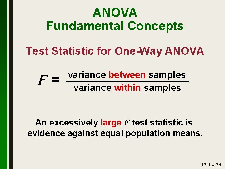
ANOVA Fundamental Concepts Test Statistic for One-Way ANOVA F= variance between samples variance within samples An excessively large F test statistic is evidence against equal population means. 12. 1 - 23

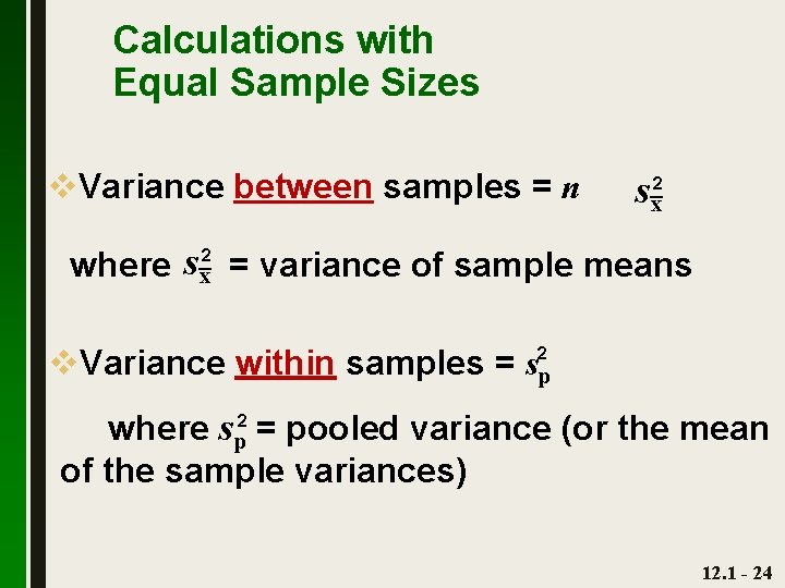
Calculations with Equal Sample Sizes v. Variance between samples = n sx 2 where sx 2 = variance of sample means v. Variance within samples = s 2 p where sp 2 = pooled variance (or the mean of the sample variances) 12. 1 - 24

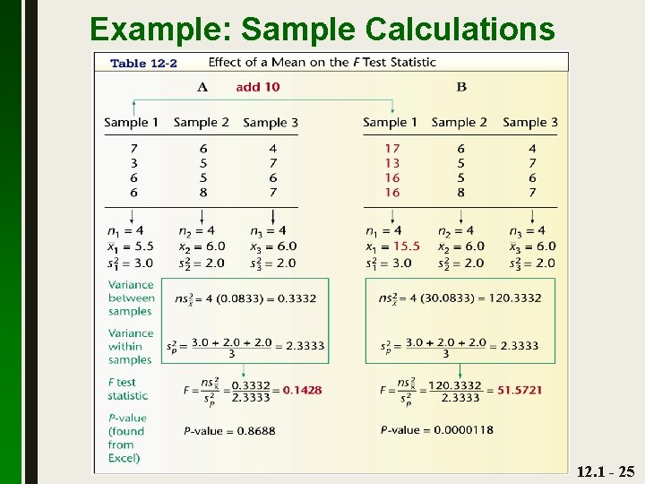
Example: Sample Calculations 12. 1 - 25

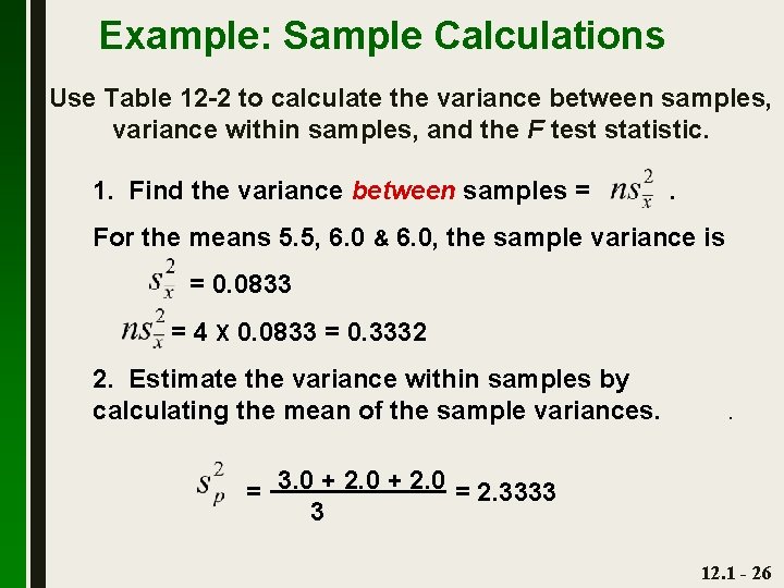
Example: Sample Calculations Use Table 12 -2 to calculate the variance between samples, variance within samples, and the F test statistic. 1. Find the variance between samples = . For the means 5. 5, 6. 0 & 6. 0, the sample variance is = 0. 0833 = 4 X 0. 0833 = 0. 3332 2. Estimate the variance within samples by calculating the mean of the sample variances. . 2. 0 + 2. 0 2. 3333 = 3. 0 + = 3 12. 1 - 26

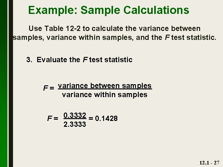
Example: Sample Calculations Use Table 12 -2 to calculate the variance between samples, variance within samples, and the F test statistic. 3. Evaluate the F test statistic F = variance between samples variance within samples F = 0. 3332 = 0. 1428 2. 3333 12. 1 - 27

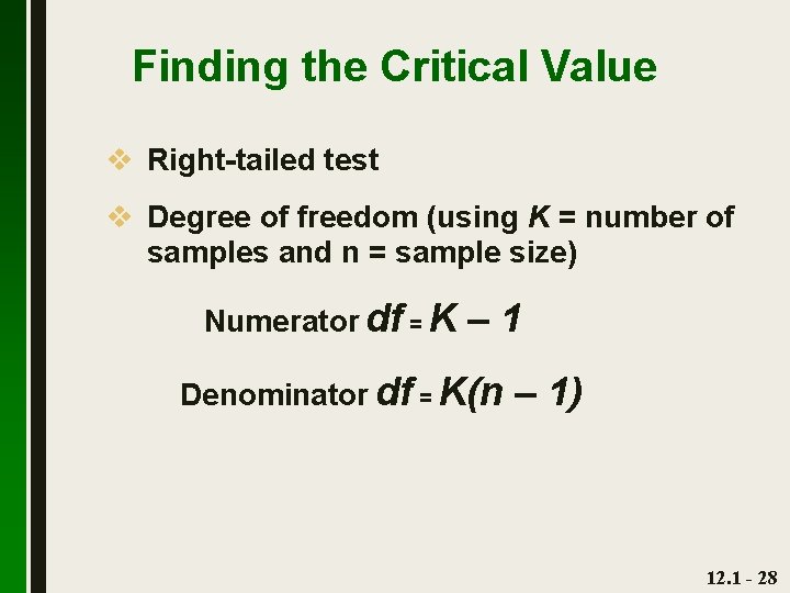
Finding the Critical Value v Right-tailed test v Degree of freedom (using K = number of samples and n = sample size) Numerator df = K – 1 Denominator df = K(n – 1) 12. 1 - 28

Finding the Critical Value - cont. For Data Set A in Table 12 -2, K= 3 and n = 4 So the df are 2 for the numerator (3 – 1), and 9 for the denominator: 3(4 – 1). With α = 0. 05, the critical F value from Table A-5 is 4. 2565 12. 1 - 29

Calculations with Unequal Sample Sizes Technology should be used to obtain the P-value for the analysis of variance. We calculate an F test statistic that is the ratio of two different estimated of the common population variance 2. With unequal sample sizes, we must use weighted measures that take the sample sizes into account. 12. 1 - 30

Identifying Which Means Are Different After conducting an analysis of variance test, we might conclude that there is sufficient evidence to reject a claim of equal population means, but we cannot conclude from ANOVA that any particular mean is different from the others. 12. 1 - 31

Identifying Means That Are Different Informal methods for comparing means 1. Construct boxplots of the different samples and examine any overlap to see if one or more of the boxplots is very different from the others. 2. Construct confidence interval estimates of the means for each of the different samples, then compare those confidence intervals to see if one or more of them doesn’t overlap with the others. 12. 1 - 32

Formal Procedures for Identifying Which Means Are Different • Range tests • Multiple comparison tests: e. g. Bonferroni test 12. 1 - 33

Bonferroni Multiple Comparison Test Step 1. Do a separate t test for each pair of samples, but make the adjustments described in the following steps. Step 2. For an estimate of the variance σ2 that is common to all of the involved populations, use the value of MS(error). 12. 1 - 34

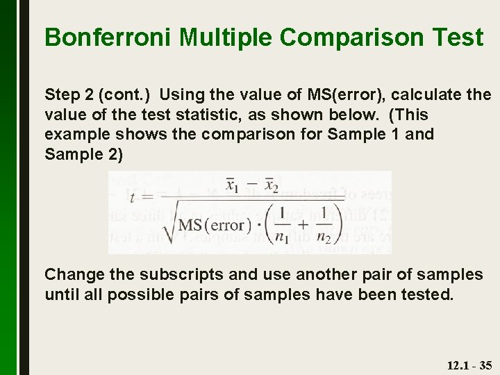
Bonferroni Multiple Comparison Test Step 2 (cont. ) Using the value of MS(error), calculate the value of the test statistic, as shown below. (This example shows the comparison for Sample 1 and Sample 2) Change the subscripts and use another pair of samples until all possible pairs of samples have been tested. 12. 1 - 35

Bonferroni Multiple Comparison Test Step 3. Find either the critical t value or the P-value, but make the following adjustment: P-value: Use the test statistic t with df = N – k, where N is the total number of sample values and k is the number of samples, and find P-value (using Table A-3 or technology), but adjust the P-value by multiplying it by the number of different possible pairings of two samples. (For example, with 3 samples, there are 3 different possible pairings, so adjust the P-value by multiplying it by 3). 12. 1 - 36

Bonferroni Multiple Comparison Test Step 3 (cont. ) Critical value: When finding the critical value, adjust the significance level α by dividing it by the number of different possible pairings of two samples. (For example, with 3 samples, there are 3 different possible pairings, so adjust the significance level by dividing it by 3). 12. 1 - 37

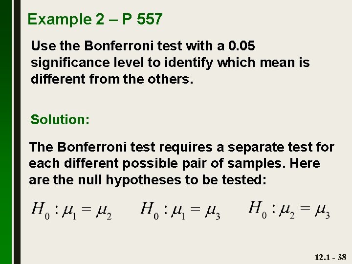
Example 2 – P 557 Use the Bonferroni test with a 0. 05 significance level to identify which mean is different from the others. Solution: The Bonferroni test requires a separate test for each different possible pair of samples. Here are the null hypotheses to be tested: 12. 1 - 38

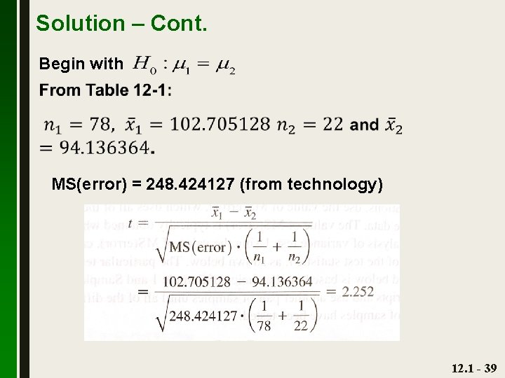
Solution – Cont. Begin with MS(error) = 248. 424127 (from technology) 12. 1 - 39

Solution – Cont. The number of degrees of freedom is df = N – k = 121 – 3 = 118. With a test statistic of t = 2. 252 and with df = 118, the two-tailed P-value is 0. 026172, but we adjust this Pvalue by multiplying it by 3 (the number of different possible pairs of samples) to get a final P-value of 0. 078516. Because this P-value is not small (less than 0. 05), we fail to reject the null hypothesis. It appears that Samples 1 and 2 do not have significantly different means. 12. 1 - 40

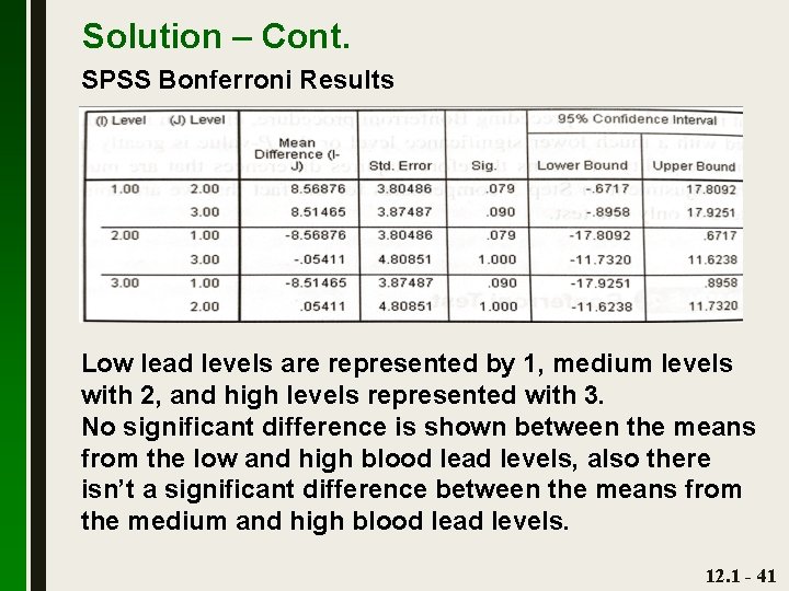
Solution – Cont. SPSS Bonferroni Results Low lead levels are represented by 1, medium levels with 2, and high levels represented with 3. No significant difference is shown between the means from the low and high blood lead levels, also there isn’t a significant difference between the means from the medium and high blood lead levels. 12. 1 - 41

THANK YOU!