Chapter 12 Advanced MicroLevel Valuation for Real Estate

Chapter 12: Advanced Micro-Level Valuation for Real Estate

Classical Corporate Finance Capital Budgeting Classical Securities Investments Analysis Unique Real Estate Factors Advanced Valuation Topics for R. E. : 1. Market Value vs Investment Value; 2. Considerations of Asset Market Inefficiency; 3. Considerations of “Dueling Asset Mkts”: 2 parallel asset mkts: Property Mkt & REIT Mkt.

12. 1: Market Value & Investment Value: 1) "MARKET VALUE" (MV) = What you can sell the asset for today. 2) "INVESTMENT VALUE" (IV) = What the asset is worth to you if you’re not going to sell it for a long time.

Market Value: • When you sell a property, you don’t know exactly what price you can get. • There is a probability distribution of the possible prices… The mean of this distribution (“expected price”) is the market value (MV) MV

Market Value: Market value is the opportunity cost (or opportunity value) of the asset, as of the given point in time. Investor gives up opportunity to retain or receive MV in cash when she decides instead to purchase or continue holding the asset. MV Any investor has the opportunity to either purchase or sell the asset at (or near) its MV (and with actual ex post transaction price as likely to be above as below the MV).

Investment Value: • Similar to “intrinsic value” or “inherent value” (based on long-term usage value of the asset), only: • Applies to a non-user owner (“landlord”), i. e. , an investor. • But ignoring current market value (“exchange value”), i. e. , assuming a long-term holding of the asset. • Defined with respect to a particular specified owner. • Based on expected future net after-tax cash flows from the asset to that particular owner/investor.

Market Value & Investment Value Summarizing the meanings… 1) "MARKET VALUE" (MV) = What you can sell the asset for today. • Equals opportunity cost/value. • Is the same for everyone (for a given asset, as of a given point in time, although there may be disagreement about what the true MV is). • Based on property-level before-tax cash flows & capital mkt OCC. 2) "INVESTMENT VALUE" (IV) = What the asset is worth to you if you’re not going to sell it for a long time. • Can be different for different investors (for the same asset as of the same point in time, due to different ability to profit from the asset). • Based on specified owner’s after-tax cash flows & capital mkt OCC.

Relationship to classical corporate finance capital budgeting: • In typical corporate cap. budgeting there is no market for the underlying physical assets, • Hence, MV does not exist, and NPV can only be measured based on IV. Label this value NPVIV. • If a publicly-traded corp. obtains NPVIV in a project, this value will rapidly be reflected in the corp’s equity MV, due to the informational efficiency of the stock market. Hence, IVCORP = MVSTOCK. ` (This applies to REITs too. ) • In real estate, existence of property market causes both MV and IV to exist directly in the underlying physical assets, but they may not be the same value (for a given investor). • Hence, both measures are of interest for real estate investment decision making (and we can compute both NPVIV and NPVMV ).

Why is IV of interest? • Because investors (& corporations) do not have to trade in the asset market in the short run. • Because real estate investors (in particular, in the direct private asset market) face high transaction costs from trading, making long holding periods desirable (to mitigate transaction cost impact on achieved multi-period annual return). Why is MV of interest? • Because it represents the current opportunity value of the investment (at least in the case of real estate assets, where there is a functioning market for the assets in question). • Because market values reflect a large amount of “intelligence” about value (“information aggregation” function of asset markets).

How to estimate MV and IV in real estate. . . • For MV: Observe transaction prices in the property market. • For IV: Use DCF: Compute AT CFs, Disc. @ AT OCC. (Normally, use a long horizon, e. g. , 10 years. ) DCF valuation also useful to estimate MV for real estate, because it underlies MV (and also for the “exercise” reason noted in Ch. 10): Disc BT CFs @ BT OCC. But DCF estimation of MV must be “calibrated” to marginal investors in current property market (to arrive at correct MV, reflecting current mkt pricing). DCF estimation is more necessary to estimate IV than MV (IV cannot be empirically observed, because it is unique to each investor). Long-term CF forecast is only way to estimate IV: Disc AT CFs @ AT OCC.

Estimating investment value: Best practice. . . • DCF numerators (CFs) should be “personalized” to reflect incremental after-tax CF effects for the specified investor. • DCF denominators (OCCs) should NOT be personalized; They should reflect the capital market’s OCC, only on an after-tax basis (i. e. , reflecting the tax rate of the marginal investor in the relevant capital market). Why? . . . • OCC reflects “price of time” & “price of risk” (i. e. , value of trade-off betw $ today vs $ tomorrow, value of trade-off betw certain $ vs uncertain $). • These prices are determined in the capital market. • All investors can always participate in the capital market. • Hence: capital market’s prices (for time & risk) always represent the relevant opportunity, for all investors, for the purpose of translating uncertain future $ into certain present $.

Estimating investment value: Best practice. . . • DCF numerators (CFs) should be “personalized” to reflect incremental after-tax CF effects for the specified investor. • DCF denominators (OCCs) should NOT be personalized; They should reflect the capital market’s OCC, only on an after-tax basis (i. e. , reflecting the tax rate of the marginal investor in the relevant capital market). Why? . . . Furthermore, suppose not. . . • This would imply, e. g. , a “personalized risk premium” in the discount rate. • This would lack rigor, and tempt abuse (e. g. , “pet project” gets low OCC). Deal with unique wealth portfolios (implying possibly unique risk premium) at macro (not micro) level: i. e. , in investor’s portfolio analysis (not in individual asset valuation).

Market Value & Investment Value… Thus, IV differs from MV because (and only because) incremental aftertax cash flows from the subject asset differ for the subject investor as compared to the marginal investor in the relevant asset market (because marginal investor determines MV). Two major causes of such differences: 1. BTCF Reason: Unique asset for unique investor enables unique profits, before-tax: (e. g. , development projects, spillover effects in adjacent parcels, corporate R. E. , sometimes some REITs? ). 2. ATCF Reason: Subject investor faces unique income tax situation, different from that of typical marginal investor in the relevant asset market (affects after-tax CFs from the property, not BTCFs).

Interaction between R. E. mkt inefficiency & the IV / MV difference. . . l Can IV MV market-wide? … (i. e. , for all investors and all properties, as of a given time) Informational inefficiency in the real estate market You can predict which way MV will change in future (better than in securities mkts). Does this imply that MV no longer well reflects fundamental long-run equilibrium value, hence MV IV (since IV is long-run holding value)?

Interaction between R. E. mkt inefficiency & the IV / MV difference. . . Can IV MV market-wide? … l CAVEAT: l This is a different conception of IV than the traditional understanding. l Real estate mkts aren’t so predictable (esp. in LR), and identifying “bubbles” is difficult in practice at the time of the bubble. l The market-wide interpretation of IV may tempt “abuse” of the IV concept: – The IV Sales Pitch (for a pet project or to close a deal): “Not to worry about the MV, the market is crazy anyway. This property is a great buy in the long run…”

In general with IV… Watch out for abuse of the concept: IV usually more subjective than MV. People have a tendency to exaggerate frequency and significance of the conditions which can cause IV MV, to argue for their interest. Be skeptical of claims that IV MV.

The market-wide IV concept can be applied to any asset class: It’s really just a “relative pricing” question… A question that can (and should) always be asked about any asset class, At the macro level.

The market-wide IV concept can be applied to any asset class: It’s really just a “relative pricing” question… A question that can (and should) always be asked about any asset class, At the macro level.

12. 1. 2: Joint Use of IV and MV in Investment Decision Making Suppose you are contemplating purchasing a property and: MV < P < IV What is NPV of the deal based on MV? Answer: NPVMV = MV – P < 0, negative. Don’t do the deal. What is NPV of the deal based on IV? Answer: NPVIV = IV – P > 0, positive. Do the deal. What should you do?

12. 1. 2: Joint Use of IV and MV in Investment Decision Making Suppose you are contemplating purchasing a property and: MV < P < IV What should you do? The conservative answer: Apply the “NPV Rule” to both IV & MV. Don’t do the deal, unless you can bargain the seller down to P = MV (which, theoretically, you should be able to do, since seller can’t expect to get more than MV from another buyer anyway: E[P] = MV): When P=MV, NPVMV= MV-P = 0, so OK. The liberal answer: Apply the “NPV Rule” only to IV. • Do the deal as long as P < IV, • Recalling that the NPV Rule says to maximize the NPV, hence, • Try to get as low a price as possible (but do the deal). And remember. . .

Remember. . . In general with IV… Watch out for abuse of the concept: IV usually more subjective than MV. People have a tendency to exaggerate frequency and significance of the conditions which can cause IV MV, to argue for their interest. Always compute and seriously consider NPVMV, and: Be skeptical of claims that IV MV.

Nevertheless, While NPVMV ≠ 0 is rare (by definition, in principle), NPVIV ≠ 0 is quite possible, not uncommon, Due to fact that IV can differ across investors. Indeed, for this reason, While NPVMV is “zero sum” across the buyer and seller: NPVMV(buyer) = -NPVMV(seller). NPVIV is not zero sum across buyer and seller: NPVIV > 0 is possible for both sides of the deal, and Finding such situations is a major objective of micro-level real estate investment activity: Searching for: NPVIV(buyer) > 0, and NPVIV(seller) > 0.

General Rule for Condition in which IV MV (Hence, NPVIV > 0 is possible): Investor(s) on at least one side of deal must be "intra-marginal". . .

Exhibit 12 -1: Relation between Investment Value (IV) and Market Value (MV) in a well-functioning asset market S $ BUYER IV ASSET PRICE=MV SELLER IV D $ = Property prices (vertical axis). Q = Volume of investment transaction per unit of time. Q 0 Q* Q Q 0 = Volume of transactions by investors with more favorable circumstances, hence would enter market at less favorable prices (i. e. , “intra-marginal” market participants, e. g. , investors with different tax circumstances than marginal investors in the market). Q* = Total volume of property transactions, including marginal investment (investors on margin are indifferent between investing and not investing in property). Note: Prices, and hence market values (MV) are determined by the IV of the marginal investors (the investors for whom NPV=0 on both an IV and MV basis).

Numerical example (drawn from Ch. 15): The Value to a Tax-Exempt Pension Fund of an Investment in Corporate Bonds L • Corp Bond Mkt Int Rate = 6% • Muni (tax-exempt) Mkt Int Rate = 4% • Eff. Tax Rate on Margl Investor in Dbt Mkt = 33%. Market for Taxed Debt Assets: S Mkt Int. Rate = 6% IVA=$101. 92=$106/1. 04 MV=$100=$106/1. 06=$104/1. 04 IVC=$99. 04=$103/1. 04 D Q 0 Q D* L = PV of a Loan (Debt Asset) in which Borrower will pay $106 next year. MV = Market Value = $100 = BTCF / (1+BTmkt. OCC) = $106/1. 06 = IV(for margl investors) = ATCF / investors (1+ATmkt. OCC) for marginal investors = $104/1. 04 = $100. investors QD IVA = Investment Value of the Corporate Bond to the Tax-Exempt Pension Fund = ATCF / (1+ATmkt. OCC) = $106/1. 04 = $101. 92. IVC = Investment Value of the Corporate Bond to a Double-Taxed Corporation (assuming corp. inc. tax rate = 33%, personal eff. tax rate on equity returns to shareholders = 25%) = ATCF / (1+ATmkt. OCC) = ($106(. 33)$6 -(. 25)$4) / 1. 04 = $103/1. 04 = $99. 04. Hence: NPV = IV-MV = -0. 96 < 0, Hence, short bonds (i. e. , borrow, don’t lend. ) Note: The issuance of one more corporate bond displaces alternative investment (or consumption) on the margin within the capital market, whether that bond happens to be sold to an intra-marginal or marginal margin investor, and whether that bond happens to be issued by an intra-marginal or marginal borrower.

Why use taxed-investor OCC in tax-exempt disc. rate to compute IV for P. F. ? . . . • Marginal corporate shareholder is a taxed individual. • Marginal pension plan member is a taxed individual. • Marginal investment of most individuals is a taxed investment (or else obtains a lower yield, like muni bonds), even though most individuals may also have tax-sheltered investments. • The ability to invest in tax-exempt vehicles that provide before-tax return levels, such as IRA or pension investments, is limited. Such investment is therfore intra-marginal. • Intra-marginal investment displaces other investment (or consumption) on the margin. Hence, this other investment (or consumption) at the margin represents the opportunity cost (what is foregone or given up) caused by the subject investment. Even if the subject investmt is intra. For these reasons, the after-tax OCC applicable to intra-marginal investment should reflect the opportunity cost of the marginal investment (in the asset market), which in turn reflects the tax rate of the marginal investor in that mkt.

Why use taxed-investor OCC in tax-exempt disc. rate to compute IV for P. F. ? . . . Suppose not. . . • Suppose discount Pension Fund after-tax cash flows @ Pension Fund after-tax OCC: • IVA = $106 / 1. 06 = $100 = MV. • NPVIV = 0 for P. F. investment, even though PF is taxadvantaged relative to marginal investor! (Recall: NPVIV=IVMV. ) • This would not make sense for Investment Value (IVs are supposed to reflect tax advantage, or disadvantage). For these reasons, the after-tax OCC applicable to intra-marginal investment should reflect the opportunity cost of the marginal investment (in the asset market), which in turn reflects the tax rate of the marginal investor in that mkt.

Thus, General Condition to allow NPV>0: It’s based on IV, not MV, and It requires “uniqueness” (“intramarginalness”). . . (For marginal investors: IV=MV. )

How to know whether you are an "intra-marginal" investor. . . "Marginal investors" are those who determine market prices. Are you similar to the types of investors who are typically buying and selling in the market (on both sides of the mkt), determining the prices at which deals are being done? If "yes", then you are not "intra-marginal".

"UNIQUENESS" is necessary for IV MV, hence for NPV>0. Therefore: NPV>0 ==> UNIQUENESS. . . So, If you think you've found a large NPV>0 deal: l Be cautious; l Look for UNIQUENESS; l If you don't find it, then you probably don't really have NPV>0 (even on the basis of IV rather than MV). Two major characteristics to look for: 1. Intra-marginal investors should be net on one side of the market or the other (either net buyers, or net sellers). 2. Intra-marginal investors should differ from the opposite parties in the deals they do (in some way significant for determining IV, possibly for subject property only), or at least they should differ from the typical marginal investor in the relevant asset market.

Most common sources of NPVIV > 0: • Unique income tax status of investor: • • • Operational advantages in controlling the real productive capacity of the property (its usage): • • • Applies to specific properties for the investor; Typically occurs in “corporate real estate” (e. g. , a unique location that is valuable for the subject corporate user but not to any other user). Space market monopoly or spillover effects: • • • Applies to all deals for the investor (non-unique properties); Typically occurs for tax-exempt (e. g. , pension funds) & double-taxed (e. g. profitable “C” corps) entities (on opposite sides). Applies to specific properties for the investor; Typically occurs for real estate developers, in devlpt projects (e. g. , ability to profit from synergy with adjacent sites already owned). Entrepreneurial profit: • • • Applies to specific properties for the investor; Occurs for “visionary” real estate developers who develop a better use for a given site (or better site for a given use) than anyone else could have imagined. Positive NPV is in site acquisition where developer’s IV is greater than anyone else’s IV for the given site, hence greater than MV of the site. Profit subsequently realized by achievement of built project’s MV.

Most common sources of NPVIV > 0: Actually, there is also another source that is not uncommon: • Differences between REIT Market valuation vs Private Asset Market valuation of real estate: • NPVIV(REIT) = IVREIT – MVPRIV = MVREIT – MVPRIV , for REIT buying, • NPVIV(REIT) = MVPRIV – IVREIT = MVPRIV – MVREIT , for REIT selling. (See Section 12. 3. )

12. 2: Danger and Opportunity in Market Inefficiency. . . In private asset markets, unique, whole assets are traded infrequently, sometimes without public disclosure of price. High transaction costs & fuzzy information prevents arbitrage. As a result: Private real estate asset markets are less “informationally efficient” than public securities markets (the “price discovery” & “information aggregation” functions of the asset market are less effective). “Noisy prices” & inertia in asset market values. prices inertia

Causes (or sources) of real estate “transaction price noise” (dispersion of prices around MV): • Difficulty in “price discovery”: Unique, whole assets trade infrequently & privately (betw 2 parties only) – MV difficult to directly observe. • 2 parties in negotiation may have different: • Information, • Negotiating ability, • Motivation for transaction (pressue to close deal).

Barriers to the use of real estate asset market predictability to obtain “arbitrage” profits: • Transaction costs (5% - 10% roundtrip typical, before tax). • Noisy prices (at individual deal level). • Imperfect predictability of asset mkt (esp. in LR, yet LR holding necessary to mitigate high transaction costs). These barriers are fundamentally what enables (or causes) the sluggishness & predictability in the asset market values.

Dangers: l Because of “noisy prices” (imprecise observation of market value at the micro-level): – NPVMV ≠ 0 is possible in direct private real estate investing (that is, even based on market value), i. e. : l l You cannot rely on the efficiency of the market to protect you from buying at too high a price, or selling at to low a price. Because of “inertia” in the asset market (“sluggish prices” “inertia” – do not fully adjust right away to reflect relevant news) Long cycles: – Overinflated market prices may endure for a long time; Overinflated – Excessively depressed market prices may endure for a long time. Excessively depressed – Danger of getting stuck forced to “buy high” &/or to “sell low”.

Opportunities: l From noise: DO YOUR “HOMEWORK” WELL, NEGOTIATE SMARTLY, YOU MAY GET A DEAL AT POSITIVE NPV. l From inertia: ANALYZE THE MARKET TO PROFIT FROM THE PREDICTABILITY THAT RESULTS FROM ITS INERTIA TO BUY LOW & SELL HIGH (“MARKET TIMING STRATEGY”), OR AT LEAST AVOID FORCED SALES IN DOWN MKTS(E. G. , BY RETAINING LIQUIDITY) (HOW? ).

General practical implication of private real estate’s market inefficiency (relative to stock exchange): It becomes more important (in order to avoid downside dangers), and more profitable (in order to obtain upside opportunities) to invest in: • “Due diligence” at the micro level (i. e. , do your “homework” carefully in investigating specific deals). • Research at the macro level (i. e. , monitor market conditions, both within R. E. over time, and betw R. E. and other asset markets, e. g. , relative ex ante yields – e. g. , in late 80 s R. E. yields were less than bond yields in spite of low & declining inflation & overbuilt space mkts).

Historical relative pricing: Yields across the asset classes…

Chapter 12 Appendix: Noise & Values in Private R. E. Asset Mkts: Basic Valuation Theory… Understand the difference between: • Inherent Value • Investment Value • Market Value • Reservation Price • Transaction Price.

Inherent Value: Maximum value a given user would be willing (and able) to pay for the subject property, if they had to pay that much for it (or, for a user who already owns the property, the minimum they would be willing to sell it for), in the absence of any consideration of the market value (“exchange value”) of the property. – Based on usage value of the property. Investment Value: Inherent value for a non-user owner (a “landlord”), i. e. , for an investor. Market Value: Most likely or expected sale price of the subject property (mean of the ex ante transaction price probability distribution). Reservation Price: Price at which a market participant will stop searching and stop negotiating for a better deal and will close the transaction. Transaction Price: Actual price at which the property trades in a given transaction. Only the last of these is directly empirically observable.

Consider a certain type of property… Consider a certain type of property • There are many individual properties, examples of the type, • With many different owners. • Because the owners are heterogeneous, there will be a wide dispersion of “inherent values” that the owners place on the properties (e. g. , like “investment value” ) because IV differs across investors. • We can represent this dispersion by a frequency distribution over the inherent values. . .

Consider a certain type of property… Consider a certain type of property • There also many non-owners of this type of property, • Potential investors. • Because these non-owners are also heterogeneous, there will be a wide dispersion of their IV values for this type of property as well. • Another frequency distribution over the inherent values. . .

Consider a certain type of property… Consider a certain type of property • There will usually be overlap between the two distributions. . . • It makes sense for the owners’ distribution to be centered to the right of the non-owners’ distribution, because of past selection: • Those who have placed higher values on the type of property in question are more likely to already own some of it.

Because there is overlap, there is scope for trading of assets. (Recall from Ch. 7 how investor heterogeneity underlies the investment industry. ) There is a mutual benefit from some non-owners whose IV values exceed those of some owners getting together and trading: • A price (P) can be found such that: IV(owner) < P < IV(non-owner). NPVIV(non-owner) = IV(non-owner) – P > 0 NPVIV(owner) = P - IV(owner) > 0

Because there is overlap, there is scope for trading of assets. The number of non-owners willing to trade equals the area under the nonowner distribution to the right of the trading price. The number of owners willing to trade equals the area under the owner distribution to the left of the trading price. If permitted in the society, a real estate asset market will form and begin operation. . .

Inherent values tend to be widely dispersed, reflecting investor heterogeneity. The operation of the asset mkt creates “price discovery” & “information aggregation”, which causes agents’ “reservation prices” (the price at which they will stop searching or negotiating and trade) to collapse around the midpoint of the overlap, the “mkt clearing price” (MV). (Less interested owners & non-owners effectively drop out of the distributions. )

Inherent Values

Reservation Prices

Reservation Prices are influenced not only by agents’ inherent values and perceptions of the market value, but also by agents’ search costs and degree of certainty about their value perceptions.

Market Value equals market clearing price, at which number of buyers (to right of price under buyer distribution). . .

Market Value equals market clearing price, at which number of buyers (to right of price under buyer distribution) equals number of sellers (to left of price under seller distribution).

The more “informationally efficient” is the asset market, the more effective is the price discovery and the information aggregation. The market learns from itself (about the value of the type of asset being traded in the market). In the extreme, the distributions on both sides of the market (the buyers and the sellers) will collapse onto the single, market-clearing price, at which the number of buyers equals the number of sellers: Hence, observed prices exactly equal market values. This is approximately what happens in the stock market.

Real estate markets are not that informationally efficient. There is price dispersion. Recall. . . The mean of this distribution (“expected price”) is the market value (MV) MV Observed transaction prices are distributed around the market value.

It is impossible to know exactly what is the market value of any property at any point in time. Observed prices are “noisy” indications of value. MV can be estimated by observing the distribution of transaction prices, using statistical or appraisal techniques. MV can be estimated more accurately: • The larger the number of transactions (more frequent trading, “denser market”), & MV • The more homogeneous the assets traded in the mkt. • Nevertheless. . . All estimates of MV (whether appraisal or statistical) contain “error”.

Summarizing. . .

How big is random noise or error in real estate prices and value estimates? . . . There is some statistical and clinical evidence that for typical properties such noise or error has a magnitude of around 5% to 10% of the property value. That is: Std. Dev. [ε] = 5% to 10% (price dispersion) Std. Dev. [u] = 5% to 10% (appraisal dispersion) Probably larger for more unique properties. -5% +5% MV

12. 3: “Dueling” Asset Markets: The REIT Mkt vs the Private Direct Property Mkt

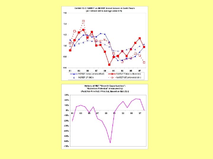
The exhibit displays the NAREIT share price level index and NCREIF appreciation level index, both de-trended and normalized to have average value of zero and standard deviation of one.

Source: Authors’ estimates based on NAREIT Index and NCREIF Index. (NCREIF cash flows are based on NOI, NAREIT cash flows are based on dividends paid out. )

The point is. . . • REIT-based valuations & private property mkt-based valuations appear to be different much of the time. • These differences do not appear to be explainable by differences in the underlying operating cash flows of the REITs vs the private properties; nor are they explainable entirely by purely firm-level considerations (e. g. , entity-level mgt, trading). • Thus, these differences appear to be genuine micro-level valuation differences, differences in the two markets’ perceptions of the values of the same underlying properties as of the same point in time. • There is some evidence that REIT valuations tend to be a bit more volatile, and to lead the private property market valuations in time (based on timing of major cyclical turning points, the lead may be up to 3 years. )

Major investment issues of the valuation difference: 1. Which market should the investor use to make real estate investments: public (REIT), or private (direct property)? 2. Is there scope for “arbitrage” between the two markets? That is, can (nearly) riskless profits be earned by moving assets from one ownership form to the other: • • Taking private assets public via REIT acquisition or IPO? ; Taking REIT assets private via buyout/privatization or simply via sale of assets or debt in the private market)? 3. What is the nature and magnitude of the micro-level differential valuation (and which value is “correct”)? In Chapter 12 we focus primarily on the 3 rd of these issues.

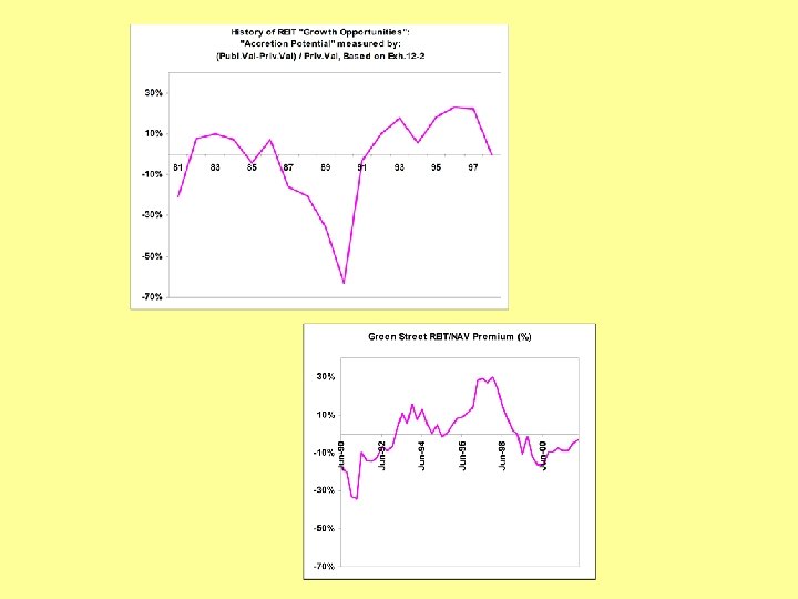
Definition of the valuation difference: For specific individual properties: IVREIT ≠ MVPRIV (Recall that stock mkt makes: IVREIT=MVREIT in share price. Thus, if a micro-level valuation difference exists, then profitable (NPV > 0) opportunities exist by buying or selling properties in the private property market. This is often referred to as (positive or negative) “accretion” opportunity for REITs: REIT Buying: NPVMV(REIT) = NPVIV(REIT) = IVREIT – MVPRIV REIT Selling: NPVMV(REIT) = NPVIV(REIT) = MVPRIV - IVREIT Mitigated by transaction costs and management considerations.

When REIT valuation > Private valuation (positive REIT premium to NAV): • REITs have growth opportunities (NPV>0, “accretion”) from buying in the private market. • REITs raise capital by issuing stock in the public mkt, use proceeds to buy properties. When REIT valuation < Private valuation (negative REIT premium to NAV): • REITs are no longer “growth stocks”, and their shares are re-priced accordingly in the stock market (price/earnings multiples fall, REITs are priced like “value stocks”, or “income stocks”). • In the extreme, REITs may become “shrinking stocks”, maximizing shareholder value by selling off property equity (or debt) and paying out proceeds in dividends. The 2 mkts swing between these 2 conditions, also with periods when they are nearly equal valued. Little “arbitrage trading” occurs when the 2 mkts are within 5%-10% of each other’s valuations (due to transaction costs). Arbitrage trading tends to keep valuation differences to less than 15%20%, but occasionally greater differences have briefly occurred.

Causes of valuation differential: Two possible sources: CFs & OCC (Recall DCF valuation formula. ) The CF-based source: Idiosyncratic valuation differences: • Affects specific properties or specific REITs. • Caused by differential ability to generate firm-level incremental CF from same properties (e. g. , REIT scale economies, franchise value, space market monopoly power, etc. ) The OCC-based source: Market-wide valuation differences: • Affects all properties, all REITs. • Reflects different informational efficiency (REIT lead). • Reflects different investor clienteles and market functioning leading to different liquidity, different risk & return patterns in the investment results, causing differential perceptions or pricing of risk. Note: Some REIT mgt actions, such as capital structure (financing of the REIT), property devlpt or trading strategy, etc. , affect firm-level REIT value but not micro-level property valuation (of existing assets in place).

Which valuation is “correct”? . . . Would you believe… They both are? (Each in their own way, for their relevant investor clientele. ) But keep in mind… • Tendency of REIT market to lead private mkt (sometimes up to 3 years). • Tendency of REIT market to exhibit “excess volatility”: • (transient “overshooting” of valuation changes, followed by “corrections”. • Two markets sometimes exhibit a “tortoise & hare” relationship.

12. 3. 5: Risk is in the object not in the beholder. (Remember from Ch. 10: Match disc. rate to the risk of the CFs being discounted. ) Property "X" has the same risk for Investor "A" as for Investor "B". Therefore, oppty cost of cap (r) is same for “A” & “B” for purposes of evaluating NPV of investment in “X” (same discount rate). Unless, say, “A” has some unique ability to alter the risk of X’s future CFs. (This is rare: be skeptical of such claims!)

Example. . . REIT A has expected total return to equity = 12%, Avg. debt int. rate = 7%, Debt/Total Asset Value Ratio = 20% What is REIT A’s (firm-level) Cost of Capital (WACC)? Ans: (0. 2)7% + (1 -0. 2)12% = 1. 4% + 9. 6% = 11%. REIT B has no debt, curr. div. yield = 6%, pays out all its earnings in dividends (share price/earnings multiple = 16. 667), avg. div. growth rate = 4%/yr. What is REIT B’s (firm-level) Cost of Capital (WACC)? [Hint: Use “Gordon Growth Model”: r = y + g. ] Ans: 6% + 4% = 10%.

Example (cont. ). . . Property X is a Boston Office Bldg, in a market where such bldgs sell at 8% cap rates (CF / V), with 0. 5% expected LR annual growth (in V & CF). It has initial CF = $1, 000/yr. How much can REIT A afford to pay for Prop. X, without suffering loss in share value, if the REIT market currently has a 10% premium over the private property market in valuation? Answer: $13, 750, 000, analyzed as follows… Prop. X Val in Priv. Mkt = $12, 500, 000 = $1, 000 / 0. 08 = $1, 000 / (8. 5% - 0. 5%), where y = r – g, as const. growth perpetuity. Prop. X Val in REIT Mkt = $12, 500, 000 * 1. 1 = $13, 750, 000, due to 10% premium. Note: “cap rate” in REIT Mkt = 1/13. 75 = 7. 27%, OCC for REIT is r. X = 7. 27% + 0. 5% = 7. 77%, i. e. : $13. 75 = $1/(. 0777 -. 05). Note: l Prop. X value for REIT is not equal to: $1, 000 / (11% - 0. 5%) = $9, 524, 000. l OCC relevant for valuing Prop. X purchase for REIT is not 11% (REIT A’s firm level WACC). l Nor is relevant OCC equal to: Prop. X OCC in Private Mkt = 8% + 0. 5% = 8. 5%.

Example (cont. ). . . Same question for REIT B. . . Answer: Same as value for REIT A: Prop. X Val for REIT B = $1, 000 / (7. 77% - 0. 5%) = $13, 750, 000. l This is not equal to $1, 000 / (10%-4%) = $1, 000 / 6% = $16, 667, 000, REIT B’s P/E multiple applied to Prop. X earnings. l Most of REIT B’s assets must be higher risk and higher growth than Prop. X (perhaps REIT B mostly does development projects). How much can Private Consortium “C” afford to pay for Prop. X? Answer: $12, 500, 000 = $1, 000 / 0. 08 = The Private Mkt’s Value. How much should either REIT (A or B) pay for Prop. X? Answer: $12, 500, 000, since that is the private mkt MV, unless they have to compete with each other (or other REITs), & the resulting bidding war bids the price up above that.

Example (1 last question. . . ) Suppose REIT B can borrow money at 6% while REIT A must pay 7% for corporate debt. Does this mean REIT B can afford to pay more for Prop. X than REIT A, assuming both REITs would finance the purchase with corporate-level debt? . . . Answer: No. • The value of the asset in the firm’s equity is unaffected by it’s corporate cost of debt. • The firm’s borrowing rate does not generally equal either its firm-level WACC or the specific OCC relevant for a given investment.