Chapter 11 TwoSample Tests of Hypothesis 1 Goals

Chapter 11 Two-Sample Tests of Hypothesis 1

Goals 1. Conduct a test of hypothesis about the difference between two independent population means when both samples have population standard deviation that are known (z) 2. Conduct a test of hypothesis about the difference between two independent population means when both samples have population standard deviation that are not known (t) 3. Conduct a test of hypothesis about the difference between two population proportions (z) 2

Compare The Means From Two Populations § Is there a difference in the mean number of defects produced on the day and the night shifts at Furniture Manufacturing Inc. ? § Comparing two means from two different populations § Is there a difference in the proportion of males from urban areas and males from rural areas who suffer from high blood pressure? § Comparing two proportions from two different populations 3

Two Populations § Two Independent Populations § E-Trade index funds § Merrill Lynch index funds § Two random samples, two sample means § Mean rate of return for E-Trade index funds (10. 4%) § Mean rate of return for Merrill Lynch index funds(11%) § Are the means different? § If they are different, is the difference due to chance (sampling error) or is it really a difference? § If they are the same, the difference between the two sample means should equal zero § “No difference” 4

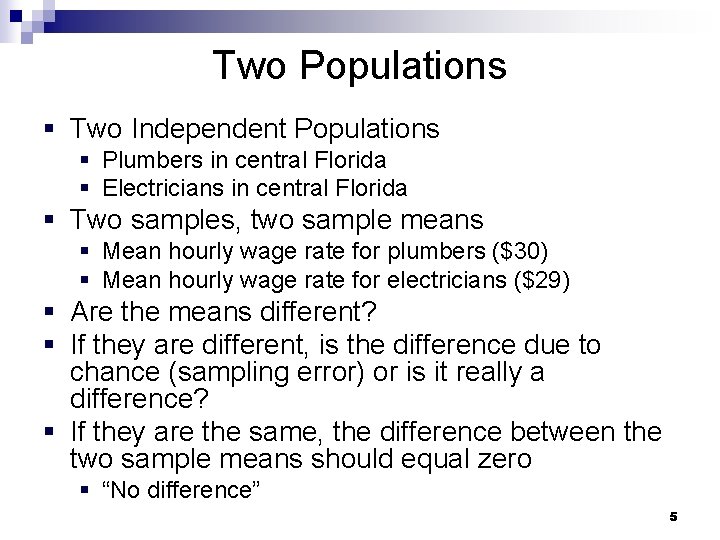
Two Populations § Two Independent Populations § Plumbers in central Florida § Electricians in central Florida § Two samples, two sample means § Mean hourly wage rate for plumbers ($30) § Mean hourly wage rate for electricians ($29) § Are the means different? § If they are different, is the difference due to chance (sampling error) or is it really a difference? § If they are the same, the difference between the two sample means should equal zero § “No difference” 5

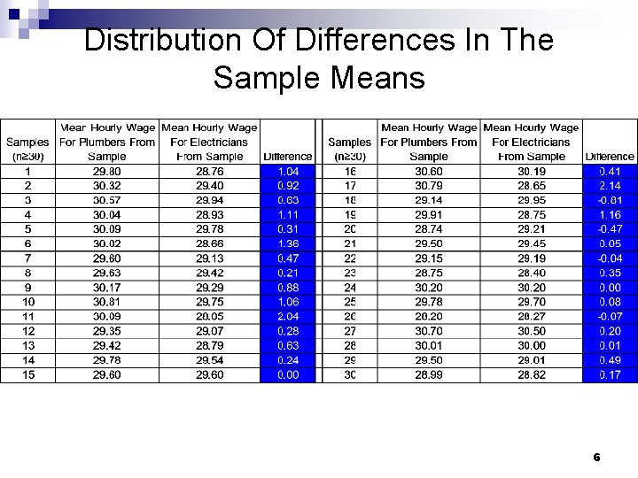
Distribution Of Differences In The Sample Means 6

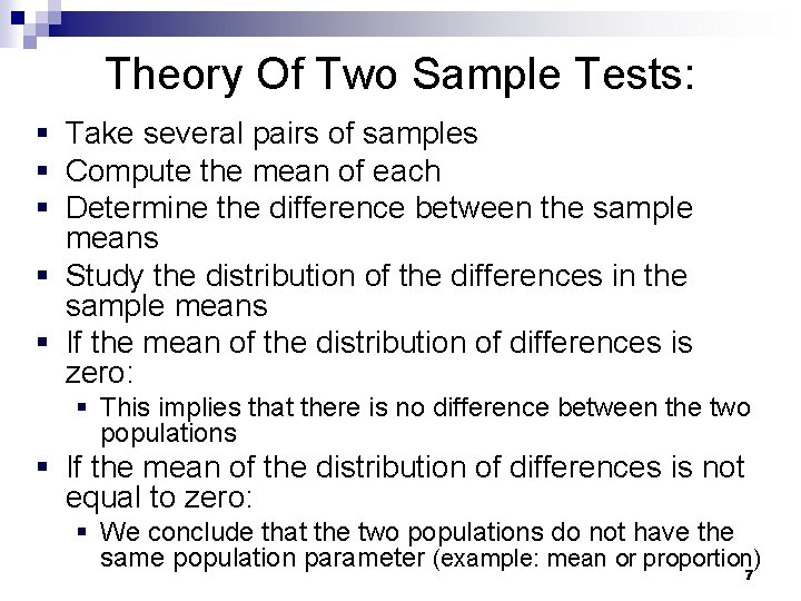
Theory Of Two Sample Tests: § Take several pairs of samples § Compute the mean of each § Determine the difference between the sample means § Study the distribution of the differences in the sample means § If the mean of the distribution of differences is zero: § This implies that there is no difference between the two populations § If the mean of the distribution of differences is not equal to zero: § We conclude that the two populations do not have the same population parameter (example: mean or proportion) 7

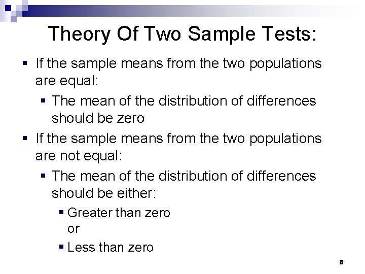
Theory Of Two Sample Tests: § If the sample means from the two populations are equal: § The mean of the distribution of differences should be zero § If the sample means from the two populations are not equal: § The mean of the distribution of differences should be either: § Greater than zero or § Less than zero 8

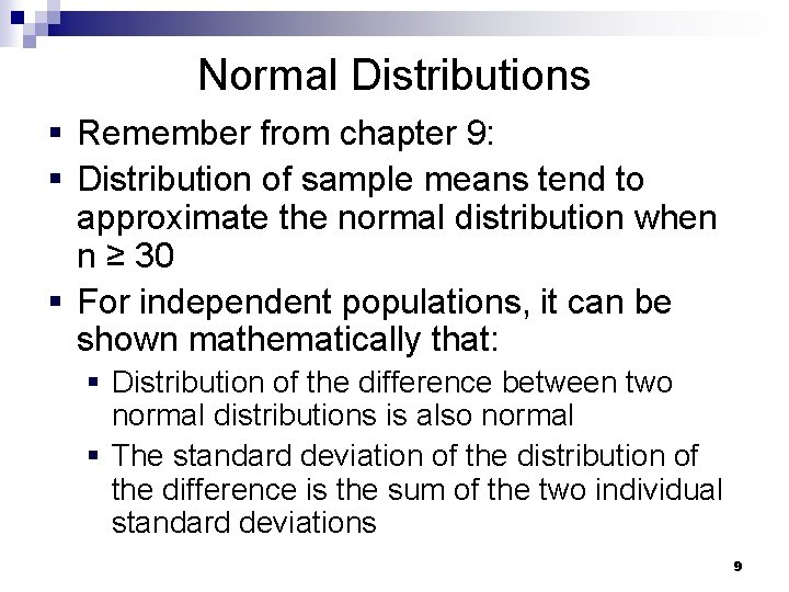
Normal Distributions § Remember from chapter 9: § Distribution of sample means tend to approximate the normal distribution when n ≥ 30 § For independent populations, it can be shown mathematically that: § Distribution of the difference between two normal distributions is also normal § The standard deviation of the distribution of the difference is the sum of the two individual standard deviations 9

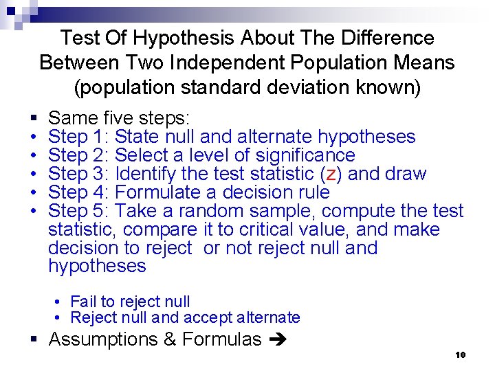
Test Of Hypothesis About The Difference Between Two Independent Population Means (population standard deviation known) § • • • Same five steps: Step 1: State null and alternate hypotheses Step 2: Select a level of significance Step 3: Identify the test statistic (z) and draw Step 4: Formulate a decision rule Step 5: Take a random sample, compute the test statistic, compare it to critical value, and make decision to reject or not reject null and hypotheses • Fail to reject null • Reject null and accept alternate § Assumptions & Formulas 10

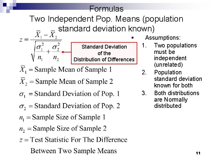
Formulas Two Independent Pop. Means (population standard deviation known) § Standard Deviation of the Distribution of Differences Assumptions: 1. Two populations must be independent (unrelated) 2. Population standard deviation known for both 3. Both distributions are Normally distributed 11

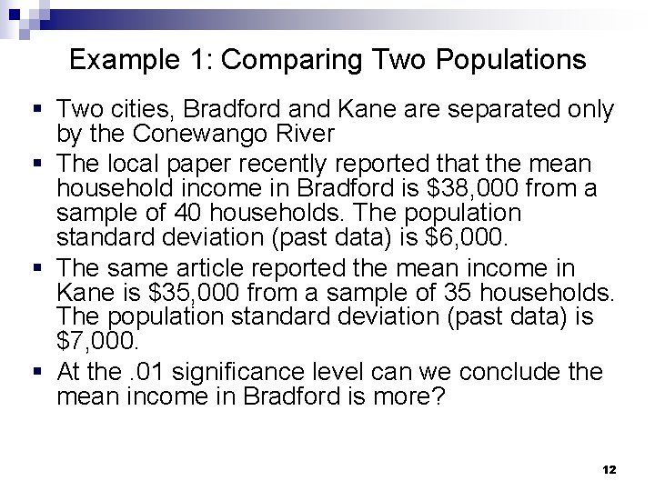
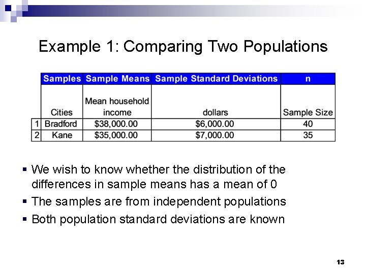
Example 1: Comparing Two Populations § Two cities, Bradford and Kane are separated only by the Conewango River § The local paper recently reported that the mean household income in Bradford is $38, 000 from a sample of 40 households. The population standard deviation (past data) is $6, 000. § The same article reported the mean income in Kane is $35, 000 from a sample of 35 households. The population standard deviation (past data) is $7, 000. § At the. 01 significance level can we conclude the mean income in Bradford is more? 12

Example 1: Comparing Two Populations § We wish to know whether the distribution of the differences in sample means has a mean of 0 § The samples are from independent populations § Both population standard deviations are known 13

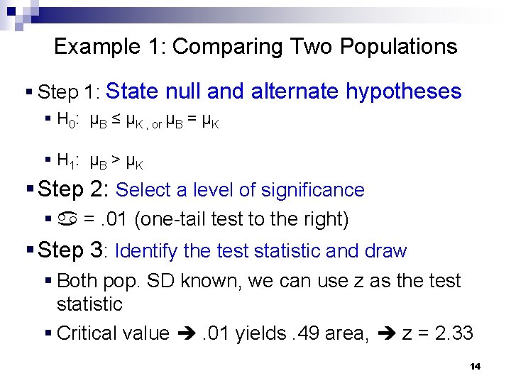
Example 1: Comparing Two Populations § Step 1: State null and alternate hypotheses § H 0: µB ≤ µK , or µB = µK § H 1: µ B > µ K § Step 2: Select a level of significance § =. 01 (one-tail test to the right) § Step 3: Identify the test statistic and draw § Both pop. SD known, we can use z as the test statistic § Critical value . 01 yields. 49 area, z = 2. 33 14

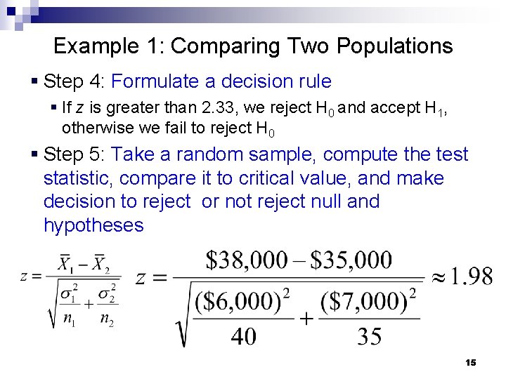
Example 1: Comparing Two Populations § Step 4: Formulate a decision rule § If z is greater than 2. 33, we reject H 0 and accept H 1, otherwise we fail to reject H 0 § Step 5: Take a random sample, compute the test statistic, compare it to critical value, and make decision to reject or not reject null and hypotheses 15

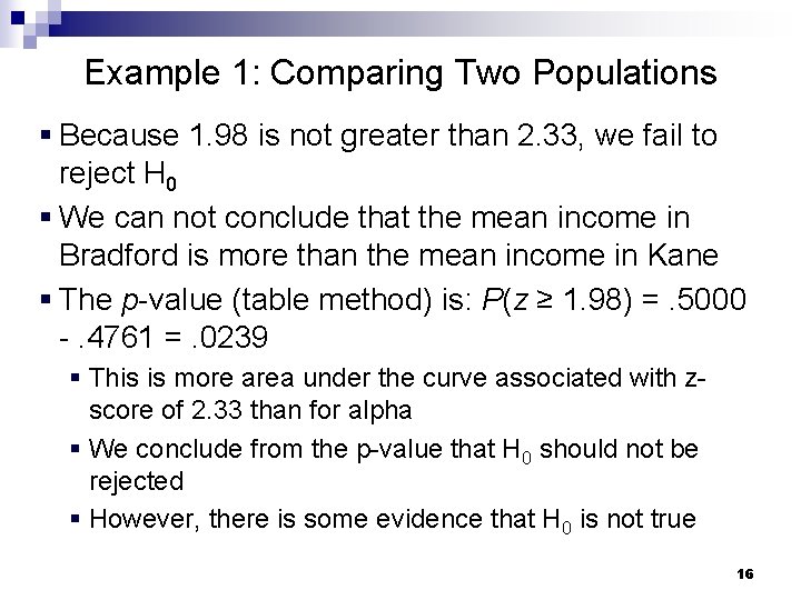
Example 1: Comparing Two Populations § Because 1. 98 is not greater than 2. 33, we fail to reject H 0 § We can not conclude that the mean income in Bradford is more than the mean income in Kane § The p-value (table method) is: P(z ≥ 1. 98) =. 5000 -. 4761 =. 0239 § This is more area under the curve associated with zscore of 2. 33 than for alpha § We conclude from the p-value that H 0 should not be rejected § However, there is some evidence that H 0 is not true 16

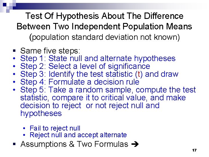
Test Of Hypothesis About The Difference Between Two Independent Population Means (population standard deviation not known) § • • • Same five steps: Step 1: State null and alternate hypotheses Step 2: Select a level of significance Step 3: Identify the test statistic (t) and draw Step 4: Formulate a decision rule Step 5: Take a random sample, compute the test statistic, compare it to critical value, and make decision to reject or not reject null and hypotheses • Fail to reject null • Reject null and accept alternate § Assumptions & Two Formulas 17

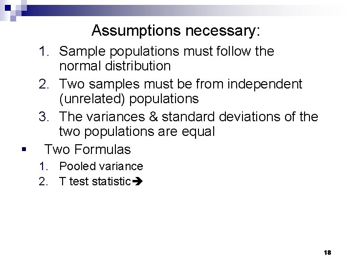
Assumptions necessary: 1. Sample populations must follow the normal distribution 2. Two samples must be from independent (unrelated) populations 3. The variances & standard deviations of the two populations are equal § Two Formulas 1. Pooled variance 2. T test statistic 18

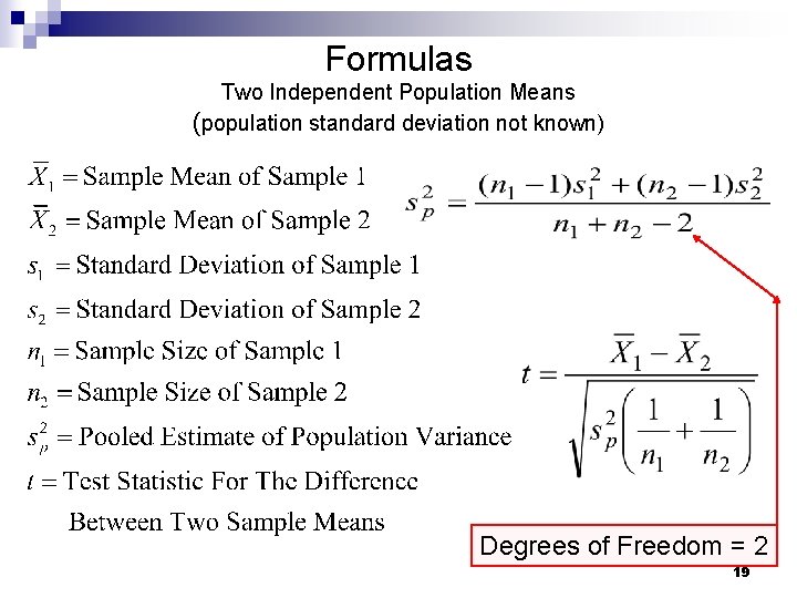
Formulas Two Independent Population Means (population standard deviation not known) Degrees of Freedom = 2 19

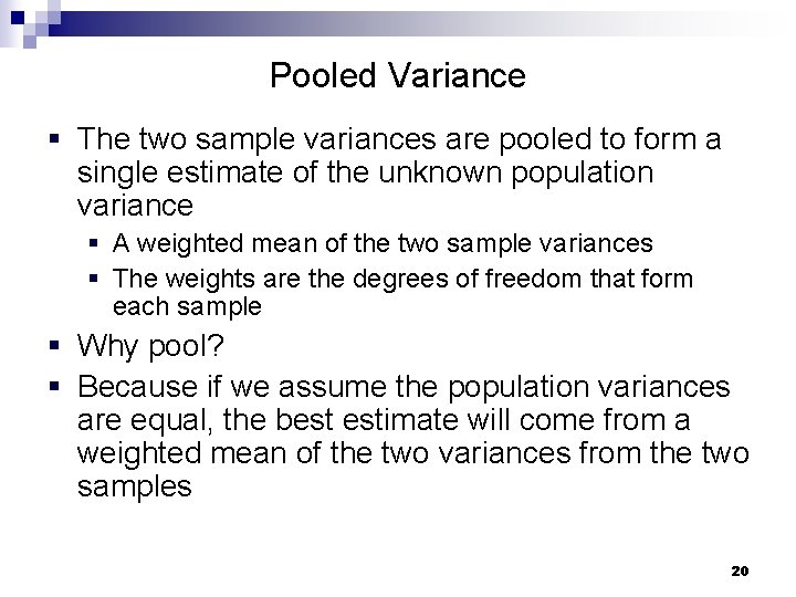
Pooled Variance § The two sample variances are pooled to form a single estimate of the unknown population variance § A weighted mean of the two sample variances § The weights are the degrees of freedom that form each sample § Why pool? § Because if we assume the population variances are equal, the best estimate will come from a weighted mean of the two variances from the two samples 20

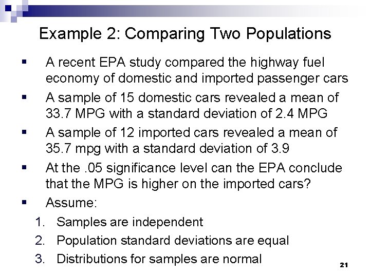
Example 2: Comparing Two Populations § § § A recent EPA study compared the highway fuel economy of domestic and imported passenger cars A sample of 15 domestic cars revealed a mean of 33. 7 MPG with a standard deviation of 2. 4 MPG A sample of 12 imported cars revealed a mean of 35. 7 mpg with a standard deviation of 3. 9 At the. 05 significance level can the EPA conclude that the MPG is higher on the imported cars? Assume: 1. Samples are independent 2. Population standard deviations are equal 3. Distributions for samples are normal 21

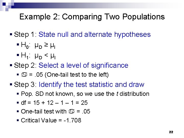
Example 2: Comparing Two Populations § Step 1: State null and alternate hypotheses § H 0: µ D ≥ µ I § H 1: µ D < µ I § Step 2: Select a level of significance § =. 05 (One-tail test to the left) § Step 3: Identify the test statistic and draw § Pop. SD not known, so we use the t distribution § df = 15 + 12 – 1 = 25 § One-tail test with =. 05 § Critical Value = -1. 708 22

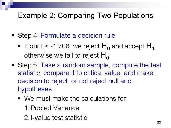
Example 2: Comparing Two Populations § Step 4: Formulate a decision rule § If our t < -1. 708, we reject H 0 and accept H 1, otherwise we fail to reject H 0 § Step 5: Take a random sample, compute the test statistic, compare it to critical value, and make decision to reject or not reject null and hypotheses § We must make the calculations for: 1. Pooled Variance 2. t-value test statistic 23

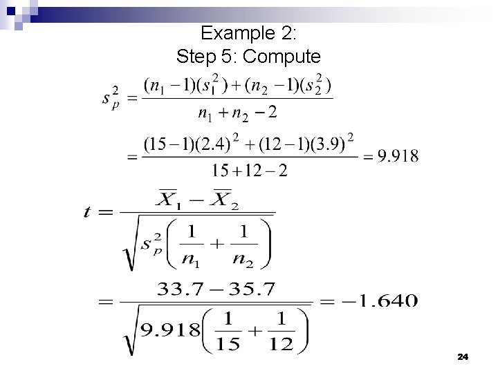
Example 2: Step 5: Compute 24

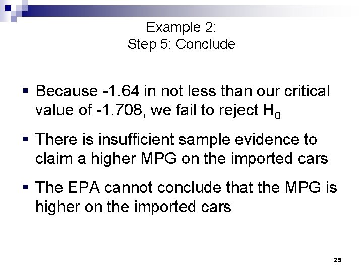
Example 2: Step 5: Conclude § Because -1. 64 in not less than our critical value of -1. 708, we fail to reject H 0 § There is insufficient sample evidence to claim a higher MPG on the imported cars § The EPA cannot conclude that the MPG is higher on the imported cars 25

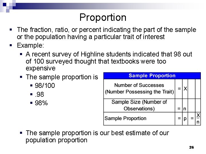
Proportion § The fraction, ratio, or percent indicating the part of the sample or the population having a particular trait of interest § Example: § A recent survey of Highline students indicated that 98 out of 100 surveyed thought that textbooks were too expensive § The sample proportion is § 98/100 §. 98 § 98% § The sample proportion is our best estimate of our population proportion 26

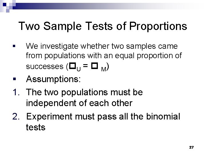
Two Sample Tests of Proportions § We investigate whether two samples came from populations with an equal proportion of successes ( U = M) § Assumptions: 1. The two populations must be independent of each other 2. Experiment must pass all the binomial tests 27

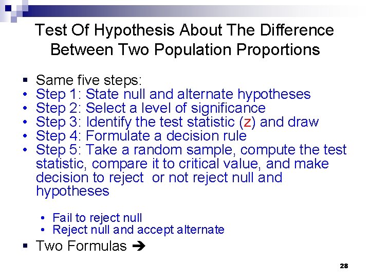
Test Of Hypothesis About The Difference Between Two Population Proportions § • • • Same five steps: Step 1: State null and alternate hypotheses Step 2: Select a level of significance Step 3: Identify the test statistic (z) and draw Step 4: Formulate a decision rule Step 5: Take a random sample, compute the test statistic, compare it to critical value, and make decision to reject or not reject null and hypotheses • Fail to reject null • Reject null and accept alternate § Two Formulas 28

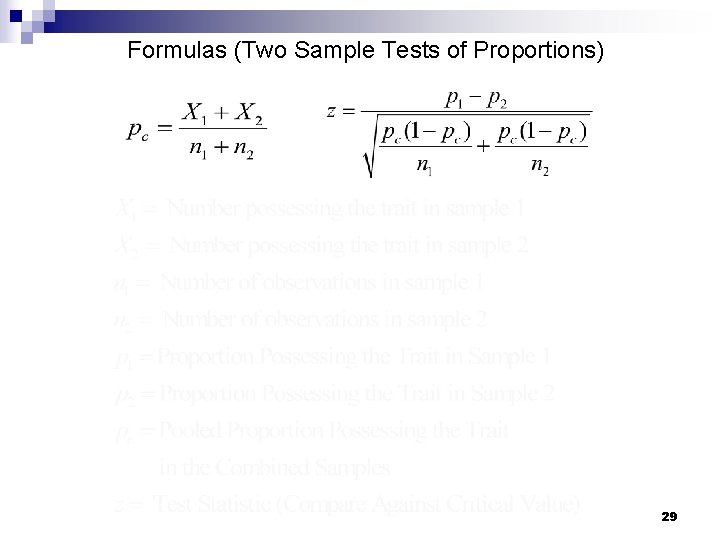
Formulas (Two Sample Tests of Proportions) 29

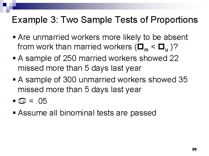
Example 3: Two Sample Tests of Proportions § Are unmarried workers more likely to be absent from work than married workers ( m < u )? § A sample of 250 married workers showed 22 missed more than 5 days last year § A sample of 300 unmarried workers showed 35 missed more than 5 days last year § =. 05 § Assume all binominal tests are passed 30

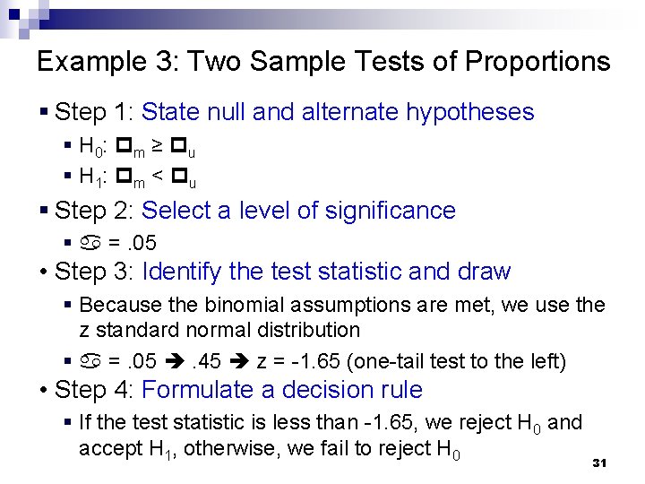
Example 3: Two Sample Tests of Proportions § Step 1: State null and alternate hypotheses § H 0: m ≥ u § H 1: m < u § Step 2: Select a level of significance § =. 05 • Step 3: Identify the test statistic and draw § Because the binomial assumptions are met, we use the z standard normal distribution § =. 05 . 45 z = -1. 65 (one-tail test to the left) • Step 4: Formulate a decision rule § If the test statistic is less than -1. 65, we reject H 0 and accept H 1, otherwise, we fail to reject H 0 31

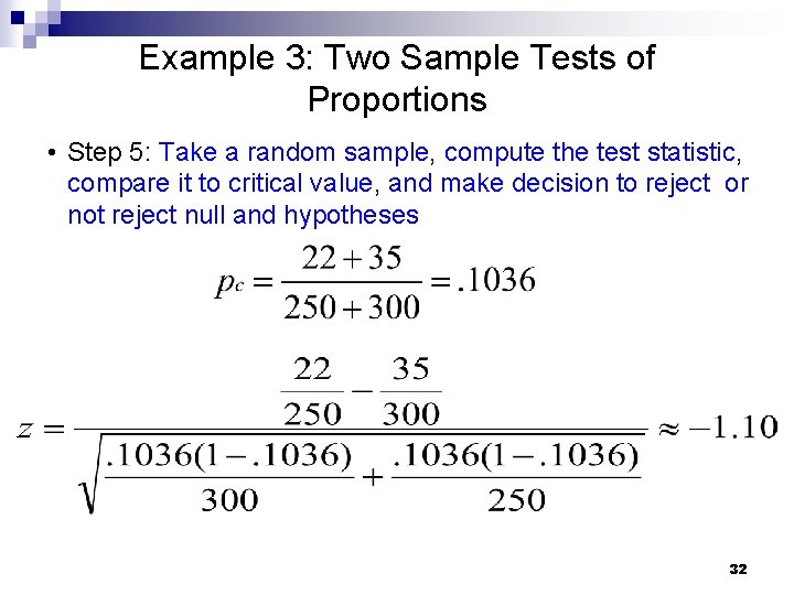
Example 3: Two Sample Tests of Proportions • Step 5: Take a random sample, compute the test statistic, compare it to critical value, and make decision to reject or not reject null and hypotheses 32

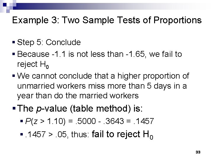
Example 3: Two Sample Tests of Proportions § Step 5: Conclude § Because -1. 1 is not less than -1. 65, we fail to reject H 0 § We cannot conclude that a higher proportion of unmarried workers miss more than 5 days in a year than do the married workers § The p-value (table method) is: § P(z > 1. 10) =. 5000 -. 3643 =. 1457 §. 1457 >. 05, thus: fail to reject H 0 33

Goals 4. Understand the difference between dependent and independent samples 5. Conduct a test of hypothesis about the mean difference between paired or dependent observations 34

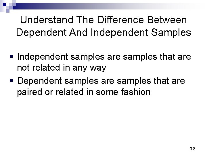
Understand The Difference Between Dependent And Independent Samples § Independent samples are samples that are not related in any way § Dependent samples are samples that are paired or related in some fashion 35

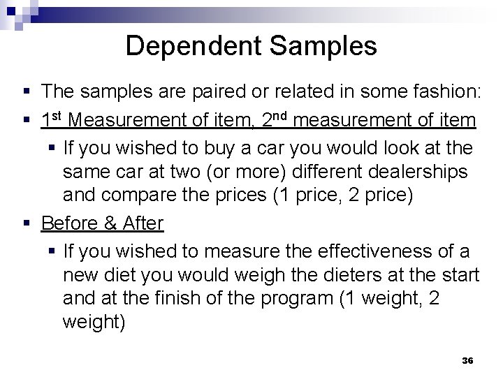
Dependent Samples § The samples are paired or related in some fashion: § 1 st Measurement of item, 2 nd measurement of item § If you wished to buy a car you would look at the same car at two (or more) different dealerships and compare the prices (1 price, 2 price) § Before & After § If you wished to measure the effectiveness of a new diet you would weigh the dieters at the start and at the finish of the program (1 weight, 2 weight) 36

Distribution Of The Differences In The Paired Values § Follows Normal Distribution § If the paired values are dependent, be sure to use the dependent formula, because it is a more accurate statistical test than the formula 11 -3 in our textbook § Formula 11 -7 helps to: § Reduce variation in the sampling distribution § Two kinds of variance (variation between 1 st & 2 nd categories for paired values, &, variation between values) are reduced to only one (variation between 1 st & 2 nd categories for paired values) § Reduced variation leads to smaller standard error, which leads to larger test statistic and greater chance of rejecting H 0 § DF will be smaller 37

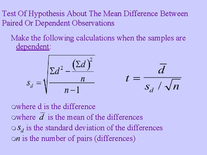
Test Of Hypothesis About The Mean Difference Between Paired Or Dependent Observations Make the following calculations when the samples are dependent: mwhere d is the difference mwhere is the mean of the differences m is the standard deviation of the differences mn is the number of pairs (differences)

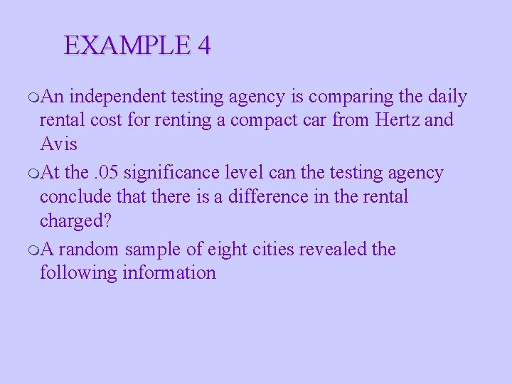
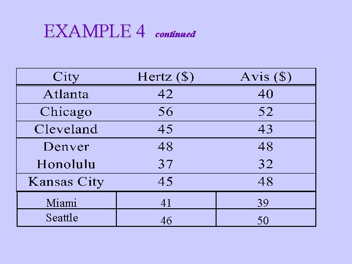
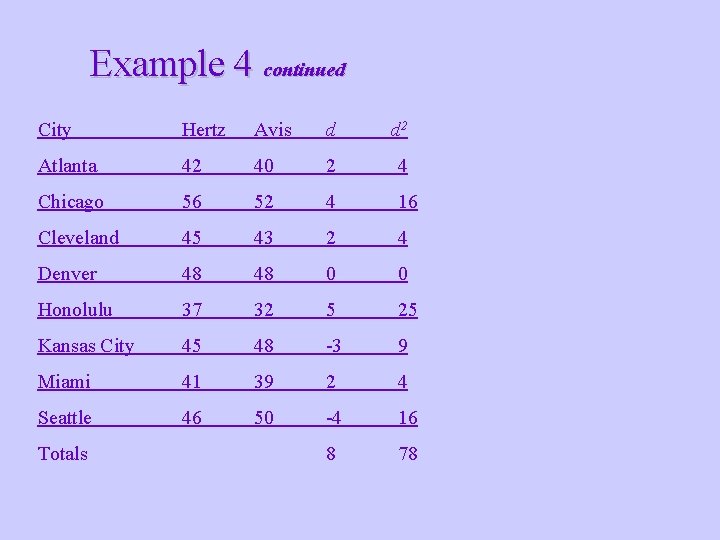
EXAMPLE 4 m. An independent testing agency is comparing the daily rental cost for renting a compact car from Hertz and Avis m. At the. 05 significance level can the testing agency conclude that there is a difference in the rental charged? m. A random sample of eight cities revealed the following information

EXAMPLE 4 Miami Seattle continued 41 39 46 50

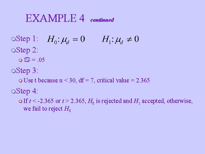
EXAMPLE 4 continued m. Step 1: m. Step 2: m m. Step =. 05 3: m Use m. Step m If t because n < 30, df = 7, critical value = 2. 365 4: t < -2. 365 or t > 2. 365, H 0 is rejected and H 1 accepted, otherwise, we fail to reject H 0

Example 4 continued City Hertz Avis d d 2 Atlanta 42 40 2 4 Chicago 56 52 4 16 Cleveland 45 43 2 4 Denver 48 48 0 0 Honolulu 37 32 5 25 Kansas City 45 48 -3 9 Miami 41 39 2 4 Seattle 46 50 -4 16 8 78 Totals

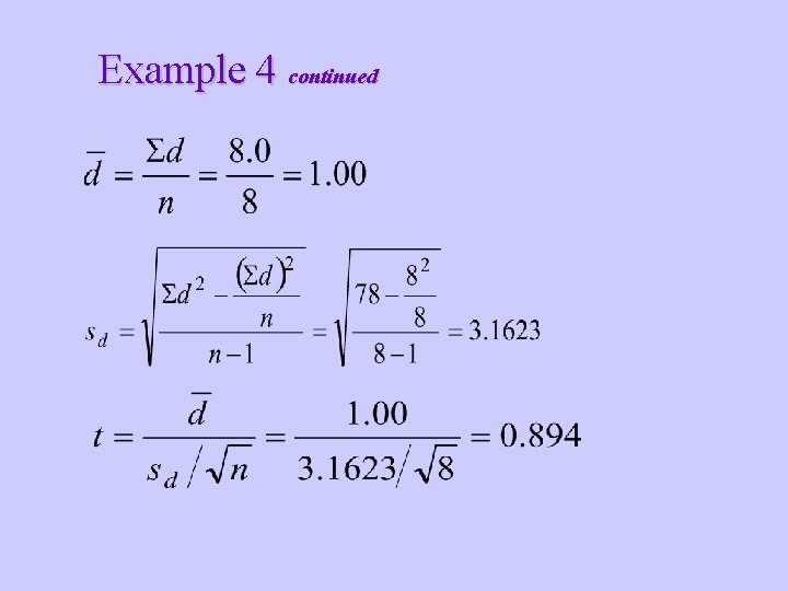
Example 4 continued

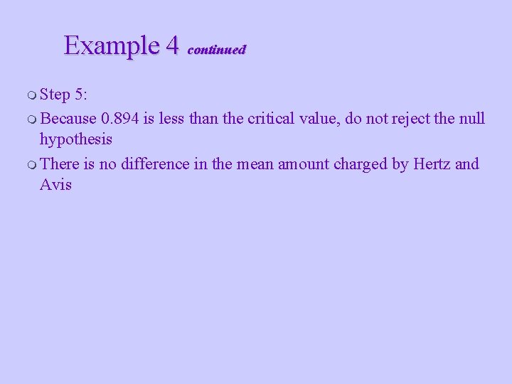
Example 4 continued m Step 5: m Because 0. 894 is less than the critical value, do not reject the null hypothesis m There is no difference in the mean amount charged by Hertz and Avis

Summarize Chapter 11 1. Conduct a test of hypothesis about the difference between two independent population means when both samples have 30 or more observations 2. Conduct a test of hypothesis about the difference between two independent population means when at least one sample has less than 30 observations 4. Conduct a test of hypothesis about the difference between two population proportions 5. Understand the difference between dependent and independent samples 6. Conduct a test of hypothesis about the mean difference between paired or dependent observations 45