Chapter 11 Statistical Inference One Sample Confidence Interval

Chapter 11 Statistical Inference: One. Sample Confidence Interval I Criticisms of Null Hypothesis Significance Testing Does not indicate whether the effect is large or small 1

Answers the wrong question: Prob(D|H 0). The correct question concerns Prob(H 0|D). Is a trivial exercise; all null hypotheses are false. Turns a continuum of uncertainty into a reject-donot reject decision. II Confidence Interval for A confidence interval for is a segment on the real number line such that has a high probability of lying on the segment. 2

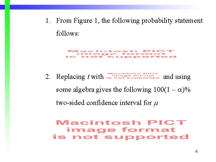
Figure 1. Sampling distribution of t. If one t statistic is randomly sampled from this population of t’s, the probability is. 95 that the obtained t will come from the interval from –t. 05/2, to t. 05/2, . 3

1. From Figure 1, the following probability statement follows: 2. Replacing t with and using some algebra gives the following 100(1 – )% two-sided confidence interval for 4

3. L 1 and L 2 denote, respectively, the lower and upper endpoints of the open confidence interval for . 4. A researcher can be 100(1 – )% confident that is greater than L 1 and less than L 2. 5. The probability (1 – ) is called the confidence coefficient and is usually equal to (1 –. 05 ) =. 95. 5

6. The assumptions associated with a confidence interval are the same as those for a one-sample t statistic. A. Computational Example: Two-Sided Interval 1. Consider the following hypotheses for the Idle-On-In College registration example: H 0: = 0 H 1: ≠ 0 6

2. A two-sided 100(1 –. 05) = 95% confidence interval for , where 7

3. The dean can be 100(1 –. 05) = 95% confident that is greater than 2. 78 and less than 3. 02. 4. The dean can be even more confident that lies in the interval from L 1 to L 2 by computing a 100(1 –. 01) = 99% confidence interval. 8

5. A two-sided 100(1 –. 01) = 99% confidence interval for , where t. 01/2, 26 = 2. 779, is given by 9

6. Graphs of the two confidence intervals 95% confidence interval for 99% confidence interval for 10

7. As the dean’s confidence that she has captured increases, so does the size of the interval from L 1 to L 2. B. More On the Interpretation of Confidence Intervals C. Computational Example: One-Sided Interval 1. Suppose that one-tailed hypotheses, H 0: ≥ 0 and H 1: < 0, reflect the dean’s hunch about the new registration procedure. 11

2. A one-sided 100(1 –. 05) = 95% confidence interval for , where 12

3. Comparison of one- and two-sided confidence intervals One-sided 95% confidence interval for Two-sided 95% confidence interval for 13

D. Advantages of Confidence Interval Estimation Over Hypothesis Testing 1. Hypothesis testing is not very informative. A confidence interval narrows the range of possible values for . 2. Confidence intervals can be used to test all null hypotheses such as H 0: = 0. Any 0 that lies outside of the confidence interval corresponds to a rejectable null hypothesis. 14

3. A sample mean and confidence interval provide an estimate of the population parameter and a range of values—the error variation—qualifying the estimate. 4. A 100(1 – )% confident interval for contains all of the values of 0 for which the null hypothesis would not be rejected. 15

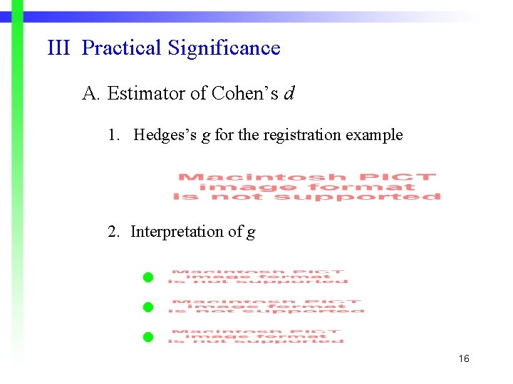
III Practical Significance A. Estimator of Cohen’s d 1. Hedges’s g for the registration example 2. Interpretation of g 16

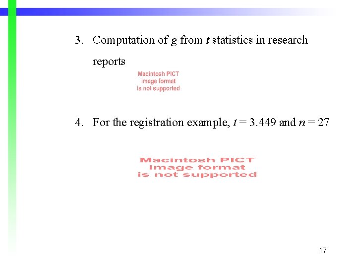
3. Computation of g from t statistics in research reports 4. For the registration example, t = 3. 449 and n = 27 17