Chapter 11 Spreadsheet Modeling and Analysis Predictive Decision

Chapter 11 Spreadsheet Modeling and Analysis

Predictive Decision Modeling � Predictive modeling is the heart and soul of business decisions. � Building decision models is more of an art than a science. � Creating good decision models requires: - solid understanding of business functional areas - knowledge of business practice and research - logical skills � It is best to start simple and enrich models as necessary.

Strategies for Predictive Decision Modeling Simple mathematics ◦ “Back-of-the-envelope” calculations can provide the basis for a more formal model Influence diagrams ◦ Introduced in Chapter 1, an influence diagram is a logical and visual representation of key model relationships

Example 11. 1: The Economic Value of a Customer �A restaurant customer dines 6 times a year and spends an average of $50 per visit. � The restaurant realizes a 40% margin on the average bill for food and drinks. � Annual gross profit on a customer = $50(6)(0. 40) = $120 � 30% of customers do not return each year. �Average lifetime of a customer = 1/0. 3 = 3. 33 years � Average gross profit during a customer’s lifetime = $120(3. 33) = $400

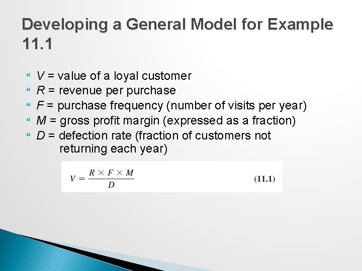
Developing a General Model for Example 11. 1 V = value of a loyal customer R = revenue per purchase F = purchase frequency (number of visits per year) M = gross profit margin (expressed as a fraction) D = defection rate (fraction of customers not returning each year)

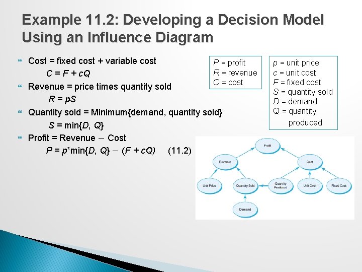
Example 11. 2: Developing a Decision Model Using an Influence Diagram Cost = fixed cost + variable cost P = profit R = revenue C = F + c. Q C = cost Revenue = price times quantity sold R = p. S Quantity sold = Minimum{demand, quantity sold} S = min{D, Q} Profit = Revenue − Cost P = p*min{D, Q} − (F + c. Q) (11. 2) p = unit price c = unit cost F = fixed cost S = quantity sold D = demand Q = quantity produced

Implementing Models on Spreadsheets Principles of good spreadsheet design: ◦ Separate the data, model calculations, and model outputs clearly in designing a spreadsheet. ◦ Do not use input data in model formulas, but reference the spreadsheet cells that contain the data. In this way, if the data change or you want to experiment with the model, you need not change any of the formulas, which can easily result in errors.

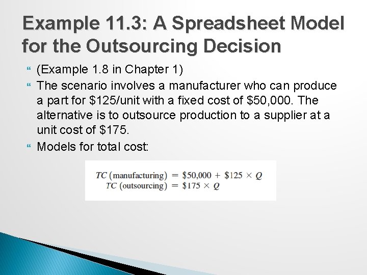
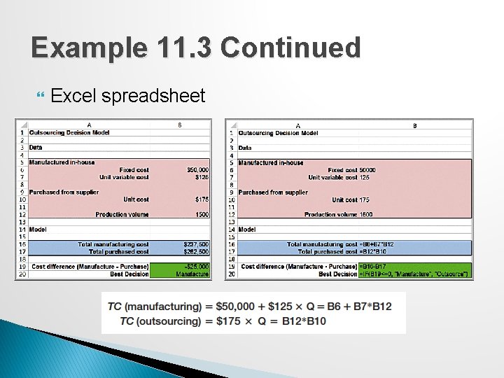
Example 11. 3: A Spreadsheet Model for the Outsourcing Decision (Example 1. 8 in Chapter 1) The scenario involves a manufacturer who can produce a part for $125/unit with a fixed cost of $50, 000. The alternative is to outsource production to a supplier at a unit cost of $175. Models for total cost:

Example 11. 3 Continued Excel spreadsheet

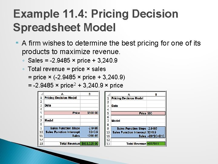
Example 11. 4: Pricing Decision Spreadsheet Model A firm wishes to determine the best pricing for one of its products to maximize revenue. ◦ Sales = -2. 9485 × price + 3, 240. 9 ◦ Total revenue = price × sales = price × (-2. 9485 × price + 3, 240. 9) = -2. 9485 × price 2 + 3, 240. 9 × price

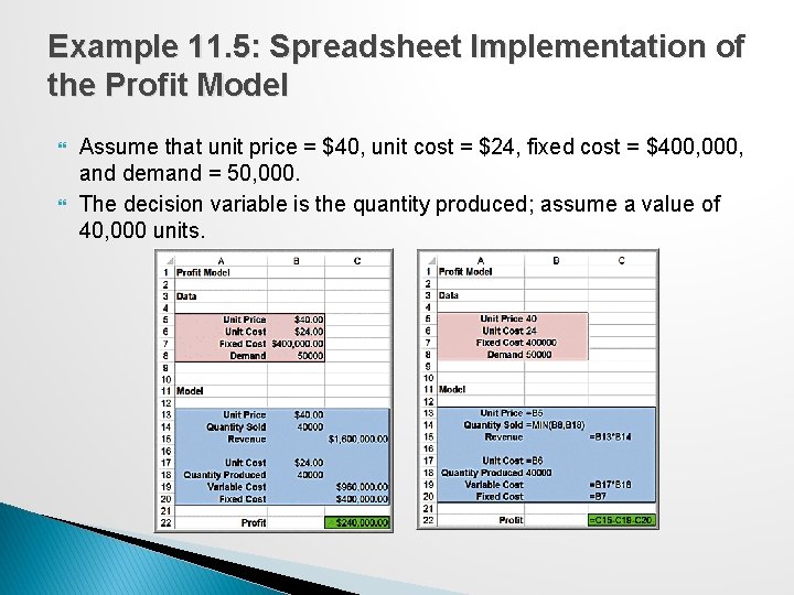
Example 11. 5: Spreadsheet Implementation of the Profit Model Assume that unit price = $40, unit cost = $24, fixed cost = $400, 000, and demand = 50, 000. The decision variable is the quantity produced; assume a value of 40, 000 units.

Spreadsheet Quality Building spreadsheet models (called spreadsheet engineering) is part and part science. Spreadsheets need to be ◦ accurate, ◦ understandable, and ◦ user friendly. Verification is the process of ensuring that a model is accurate and free from logical errors.

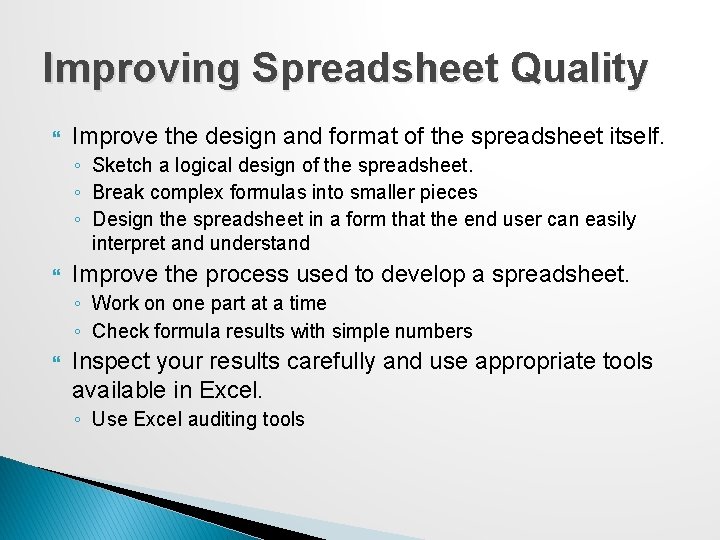
Improving Spreadsheet Quality Improve the design and format of the spreadsheet itself. ◦ Sketch a logical design of the spreadsheet. ◦ Break complex formulas into smaller pieces ◦ Design the spreadsheet in a form that the end user can easily interpret and understand Improve the process used to develop a spreadsheet. ◦ Work on one part at a time ◦ Check formula results with simple numbers Inspect your results carefully and use appropriate tools available in Excel. ◦ Use Excel auditing tools

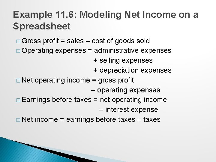
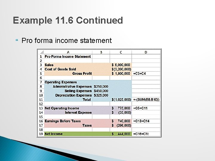
Example 11. 6: Modeling Net Income on a Spreadsheet � Gross profit = sales – cost of goods sold � Operating expenses = administrative expenses + selling expenses + depreciation expenses � Net operating income = gross profit – operating expenses � Earnings before taxes = net operating income – interest expense � Net income = earnings before taxes – taxes

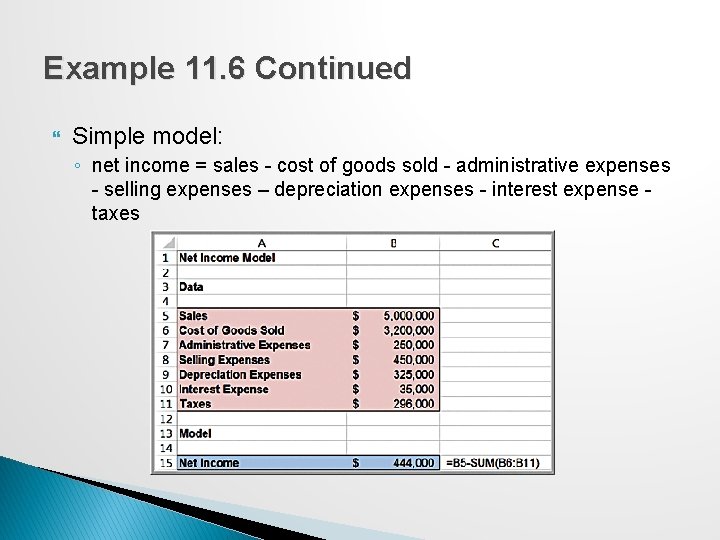
Example 11. 6 Continued Simple model: ◦ net income = sales - cost of goods sold - administrative expenses - selling expenses – depreciation expenses - interest expense taxes

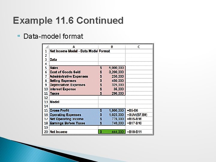
Example 11. 6 Continued Data-model format

Example 11. 6 Continued Pro forma income statement

Spreadsheet Applications in Business Analytics A wide variety of practical problems in business analytics can be modeled using spreadsheets. A useful spreadsheet model need not be complex; often, simple models can provide managers with the information they need to make good decisions.

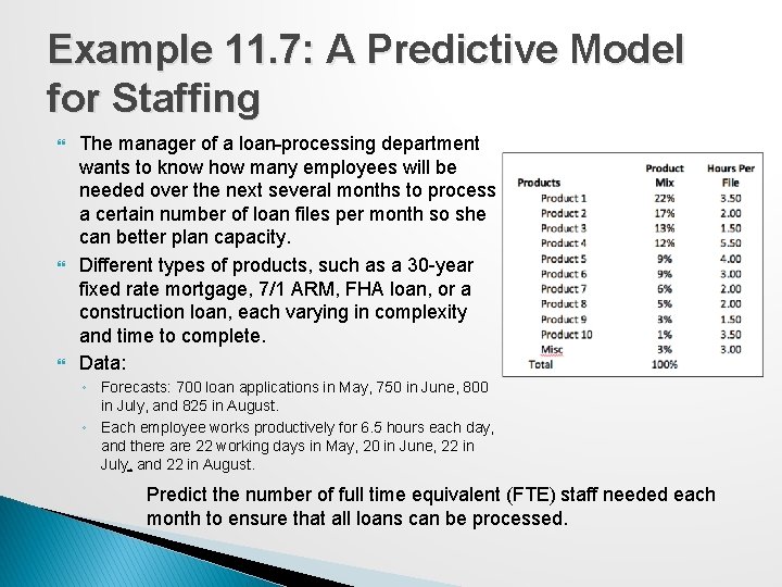
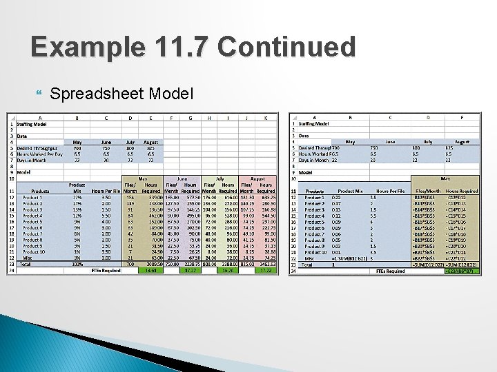
Example 11. 7: A Predictive Model for Staffing The manager of a loan processing department wants to know how many employees will be needed over the next several months to process a certain number of loan files per month so she can better plan capacity. Different types of products, such as a 30 -year fixed rate mortgage, 7/1 ARM, FHA loan, or a construction loan, each varying in complexity and time to complete. Data: ◦ Forecasts: 700 loan applications in May, 750 in June, 800 in July, and 825 in August. ◦ Each employee works productively for 6. 5 hours each day, and there are 22 working days in May, 20 in June, 22 in July, and 22 in August. Predict the number of full time equivalent (FTE) staff needed each month to ensure that all loans can be processed.

Example 11. 7 Continued Spreadsheet Model

Models Involving Multiple Time Periods Many practical models incorporate multiple time periods that are logically linked together. Taking a systematic approach to putting the pieces together logically can often make a seemingly difficult problem much easier.

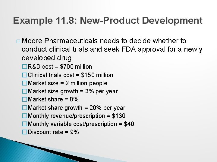
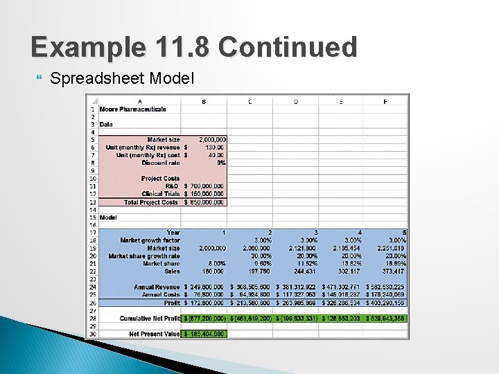
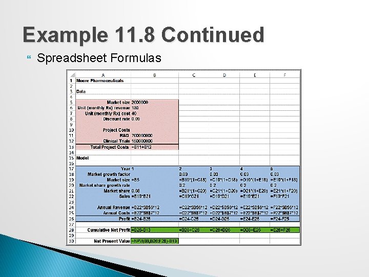
Example 11. 8: New-Product Development � Moore Pharmaceuticals needs to decide whether to conduct clinical trials and seek FDA approval for a newly developed drug. �R&D cost = $700 million �Clinical trials cost = $150 million �Market size = 2 million people �Market size growth = 3% per year �Market share = 8% �Market share growth = 20% per year �Monthly revenue/prescription = $130 �Monthly variable cost/prescription = $40 �Discount rate = 9%

Example 11. 8 Continued Spreadsheet Model

Example 11. 8 Continued Spreadsheet Formulas

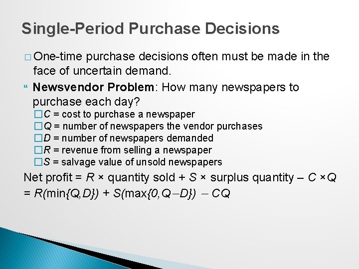
Single-Period Purchase Decisions � One-time purchase decisions often must be made in the face of uncertain demand. Newsvendor Problem: How many newspapers to purchase each day? �C = cost to purchase a newspaper �Q = number of newspapers the vendor purchases �D = number of newspapers demanded �R = revenue from selling a newspaper �S = salvage value of unsold newspapers Net profit = R × quantity sold + S × surplus quantity – C ×Q = R(min{Q, D}) + S(max{0, Q−D}) − CQ

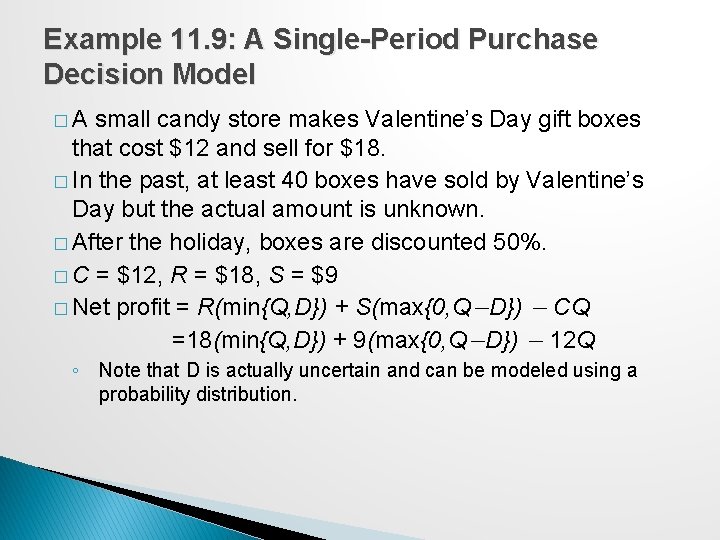
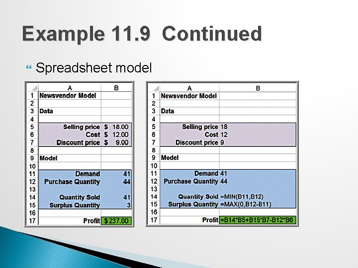
Example 11. 9: A Single-Period Purchase Decision Model �A small candy store makes Valentine’s Day gift boxes that cost $12 and sell for $18. � In the past, at least 40 boxes have sold by Valentine’s Day but the actual amount is unknown. � After the holiday, boxes are discounted 50%. � C = $12, R = $18, S = $9 � Net profit = R(min{Q, D}) + S(max{0, Q−D}) − CQ =18(min{Q, D}) + 9(max{0, Q−D}) − 12 Q ◦ Note that D is actually uncertain and can be modeled using a probability distribution.

Example 11. 9 Continued Spreadsheet model

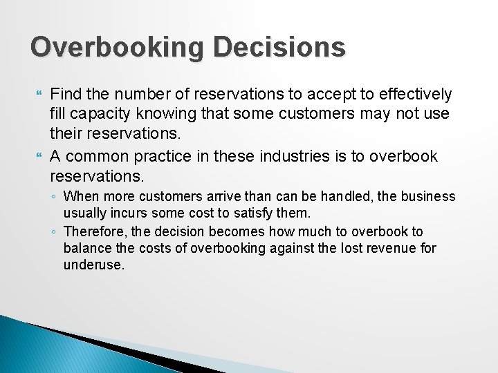
Overbooking Decisions Find the number of reservations to accept to effectively fill capacity knowing that some customers may not use their reservations. A common practice in these industries is to overbook reservations. ◦ When more customers arrive than can be handled, the business usually incurs some cost to satisfy them. ◦ Therefore, the decision becomes how much to overbook to balance the costs of overbooking against the lost revenue for underuse.

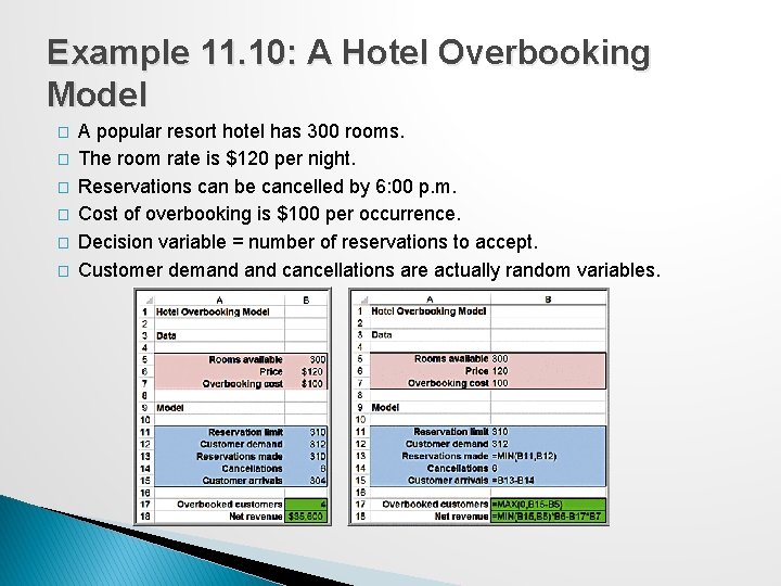
Example 11. 10: A Hotel Overbooking Model � � � A popular resort hotel has 300 rooms. The room rate is $120 per night. Reservations can be cancelled by 6: 00 p. m. Cost of overbooking is $100 per occurrence. Decision variable = number of reservations to accept. Customer demand cancellations are actually random variables.

Model Assumptions, Complexity, and Realism Models cannot capture every detail of the real problem, and managers must understand the limitations of models and their underlying assumptions. Validity refers to how well a model represents reality. Judging validity: ◦ Identify and examine the assumptions made in a model to see how they agree with our perception of the real world ◦ Compare model results to observed results

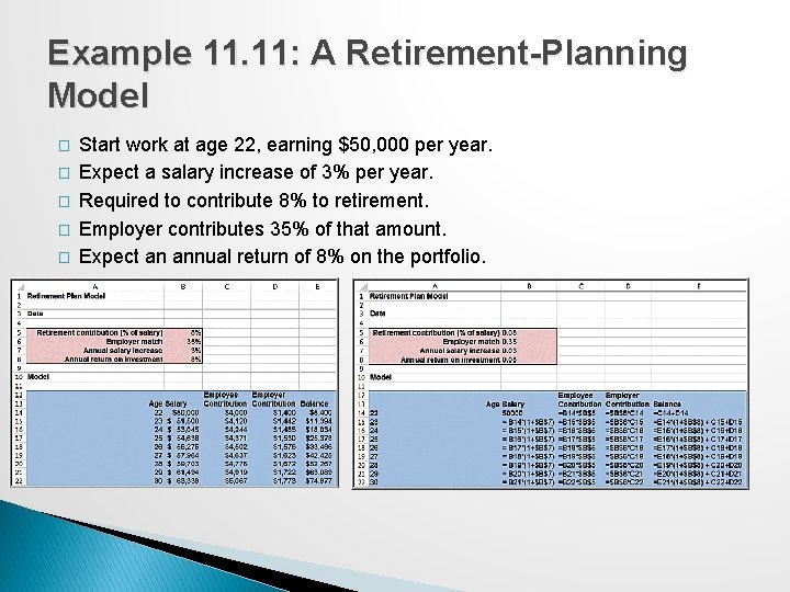
Example 11. 11: A Retirement-Planning Model � � � Start work at age 22, earning $50, 000 per year. Expect a salary increase of 3% per year. Required to contribute 8% to retirement. Employer contributes 35% of that amount. Expect an annual return of 8% on the portfolio.

Example 11. 11 Continued Validity issues: ◦ Whether the assumptions of the annual salary increase and return on investment are reasonable ◦ Whether they should be assumed to be the same each year ◦ How the model calculates the return on investment – Current year balance only? End-of-year balance plus current-year contributions? Monthly?

Data and Models Sources of data ◦ ◦ Subjective judgment Existing databases Analysis of historical data Surveys, experiments, or other methods of data collection

Using Empirical Data in Models Many predictive models in business analytics use empirical data in conjunction with logical model development. ◦ In other words, we observe some phenomenon and then try to develop a model that best reflects the data that we observe.

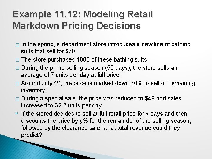
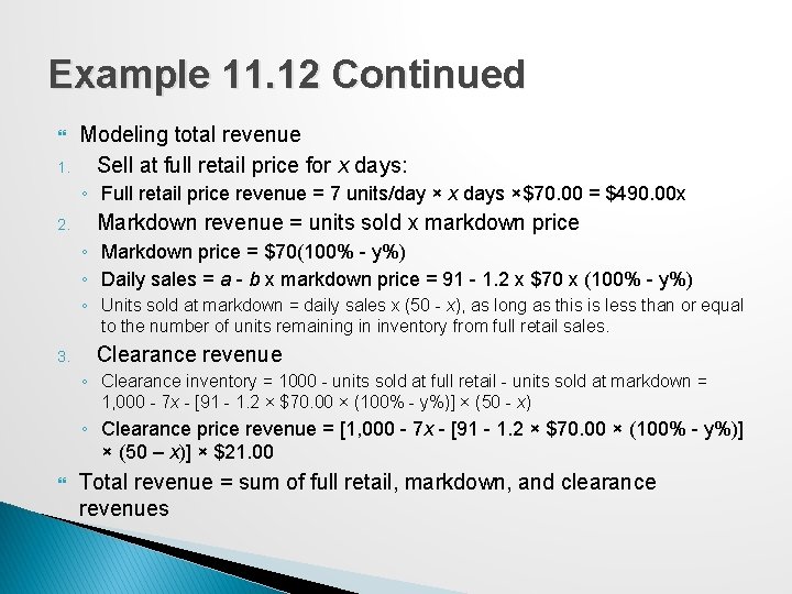
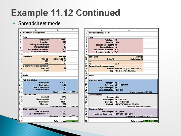
Example 11. 12: Modeling Retail Markdown Pricing Decisions � � � In the spring, a department store introduces a new line of bathing suits that sell for $70. The store purchases 1000 of these bathing suits. During the prime selling season (50 days), the store sells an average of 7 units per day at full price. Around July 4 th, the price is marked down 70% to sell off remaining inventory. During a special sale, the price was reduced to $49 and sales increased to 32. 2 units per day. If the stored decides to sell at full retail price for x days and then discounts the price by y% for the remainder of the selling season, followed by the clearance sale, what total revenue could they predict?

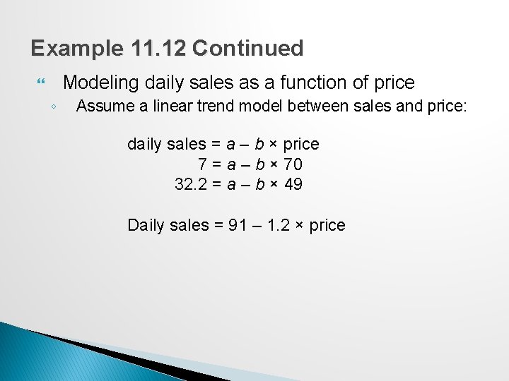
Example 11. 12 Continued Modeling daily sales as a function of price ◦ Assume a linear trend model between sales and price: daily sales = a – b × price 7 = a – b × 70 32. 2 = a – b × 49 Daily sales = 91 – 1. 2 × price

Example 11. 12 Continued 1. Modeling total revenue Sell at full retail price for x days: ◦ Full retail price revenue = 7 units/day × x days ×$70. 00 = $490. 00 x 2. Markdown revenue = units sold x markdown price ◦ Markdown price = $70(100% - y%) ◦ Daily sales = a - b x markdown price = 91 - 1. 2 x $70 x (100% - y%) ◦ Units sold at markdown = daily sales x (50 - x), as long as this is less than or equal to the number of units remaining in inventory from full retail sales. 3. Clearance revenue ◦ Clearance inventory = 1000 - units sold at full retail - units sold at markdown = 1, 000 - 7 x - [91 - 1. 2 × $70. 00 × (100% - y%)] × (50 - x) ◦ Clearance price revenue = [1, 000 - 7 x - [91 - 1. 2 × $70. 00 × (100% - y%)] × (50 – x)] × $21. 00 Total revenue = sum of full retail, markdown, and clearance revenues

Example 11. 12 Continued Spreadsheet model

Developing User-Friendly Applications Useful Excel tools ◦ Data validation ◦ Range Names ◦ Form Controls

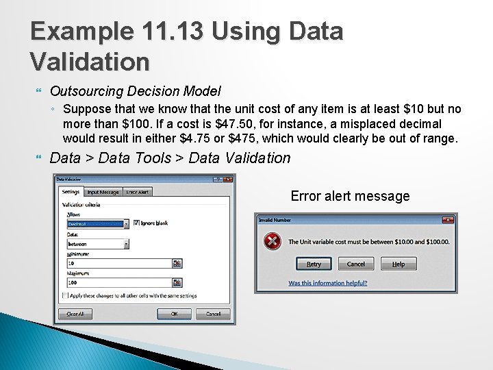
Example 11. 13 Using Data Validation Outsourcing Decision Model ◦ Suppose that we know that the unit cost of any item is at least $10 but no more than $100. If a cost is $47. 50, for instance, a misplaced decimal would result in either $4. 75 or $475, which would clearly be out of range. Data > Data Tools > Data Validation Error alert message

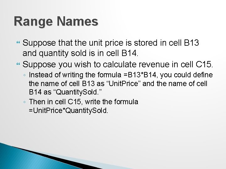
Range Names Suppose that the unit price is stored in cell B 13 and quantity sold is in cell B 14. Suppose you wish to calculate revenue in cell C 15. ◦ Instead of writing the formula =B 13*B 14, you could define the name of cell B 13 as “Unit. Price” and the name of cell B 14 as “Quantity. Sold. ” ◦ Then in cell C 15, write the formula =Unit. Price*Quantity. Sold.

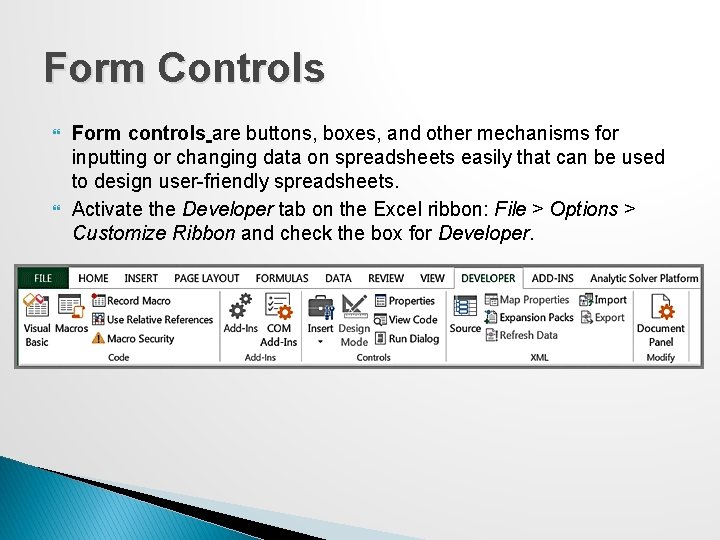
Form Controls Form controls are buttons, boxes, and other mechanisms for inputting or changing data on spreadsheets easily that can be used to design user-friendly spreadsheets. Activate the Developer tab on the Excel ribbon: File > Options > Customize Ribbon and check the box for Developer.

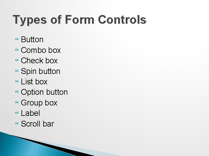
Types of Form Controls Button Combo box Check box Spin button List box Option button Group box Label Scroll bar

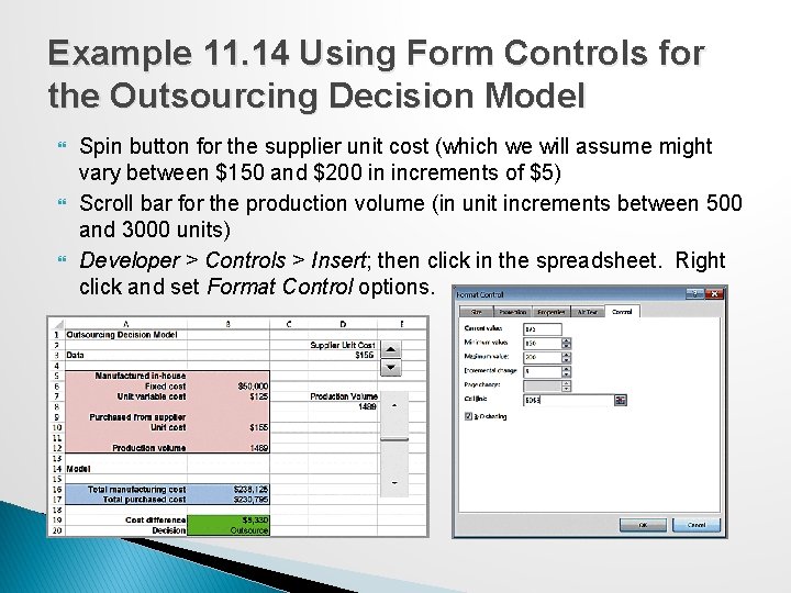
Example 11. 14 Using Form Controls for the Outsourcing Decision Model Spin button for the supplier unit cost (which we will assume might vary between $150 and $200 in increments of $5) Scroll bar for the production volume (in unit increments between 500 and 3000 units) Developer > Controls > Insert; then click in the spreadsheet. Right click and set Format Control options.

Analyzing Uncertainty and Model Assumptions Predictive analytical models are based on assumptions about the future and incorporate variables that most likely will not be known with certainty. It is usually important to investigate how these assumptions and uncertainty affect the model outputs.

What-If Analysis Spreadsheet models allow you to easily evaluate what-if questions by changing input values and recalculating model outputs. Systematic approaches to what-if analysis that are available in Excel make the process easier and more useful. ◦ Data tables ◦ Scenario Manager ◦ Goal Seek

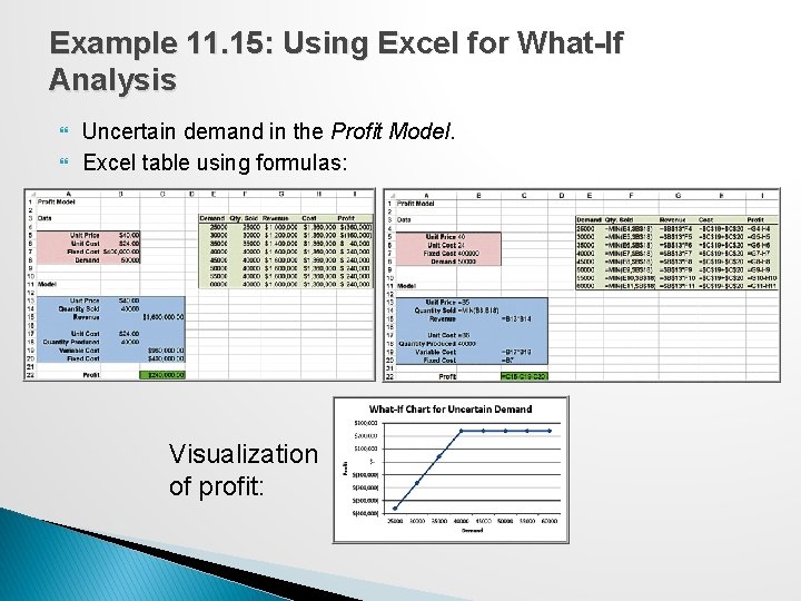
Example 11. 15: Using Excel for What-If Analysis Uncertain demand in the Profit Model. Excel table using formulas: Visualization of profit:

Data Tables � Data Tables summarize the impact of one or two inputs on a specified output. ◦ A one-way data table evaluates an output variable over a range of values for a single input variable. ◦ Two-way data tables evaluate an output variable over a range of values for two different input variables.

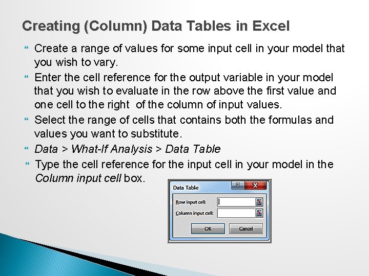
Creating (Column) Data Tables in Excel Create a range of values for some input cell in your model that you wish to vary. Enter the cell reference for the output variable in your model that you wish to evaluate in the row above the first value and one cell to the right of the column of input values. Select the range of cells that contains both the formulas and values you want to substitute. Data > What-If Analysis > Data Table Type the cell reference for the input cell in your model in the Column input cell box.

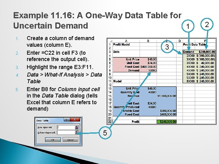
Example 11. 16: A One-Way Data Table for Uncertain Demand 1 1. 2. 3. 4. 5. Create a column of demand values (column E). Enter =C 22 in cell F 3 (to reference the output cell). Highlight the range E 3: F 11. Data > What-If Analysis > Data Table Enter B 8 for Column input cell in the Data Table dialog (tells Excel that column E refers to demand) 3 5 2

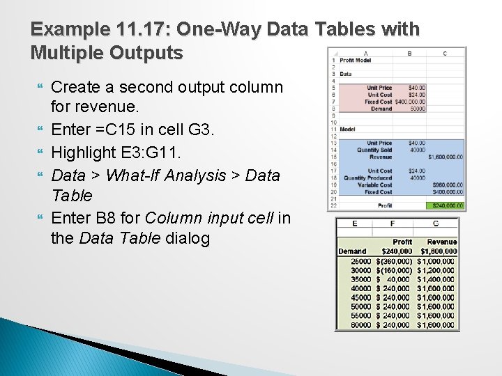
Example 11. 17: One-Way Data Tables with Multiple Outputs Create a second output column for revenue. Enter =C 15 in cell G 3. Highlight E 3: G 11. Data > What-If Analysis > Data Table Enter B 8 for Column input cell in the Data Table dialog

Two-Way Data Tables Type a list of values for one input variable in a column and a list of input values for the second input variable in a row, starting one row above and one column to the right of the column list. In the cell in the upper left-hand corner immediately above the column list and to the left of the row list, enter the cell reference of the output variable you wish to evaluate. Select the range of cells that contain this cell reference and both the row and column of values. In the Row input cell of the dialog box, enter the reference for the input cell in the model that corresponds to the input values in the row. In the Column input cell box, enter the reference for the input cell in the model that corresponds to the input values in the column.

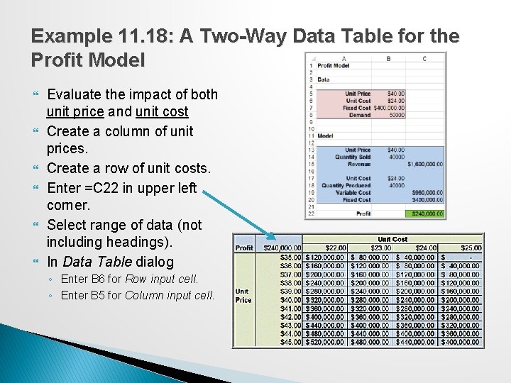
Example 11. 18: A Two-Way Data Table for the Profit Model Evaluate the impact of both unit price and unit cost Create a column of unit prices. Create a row of unit costs. Enter =C 22 in upper left corner. Select range of data (not including headings). In Data Table dialog ◦ Enter B 6 for Row input cell. ◦ Enter B 5 for Column input cell.

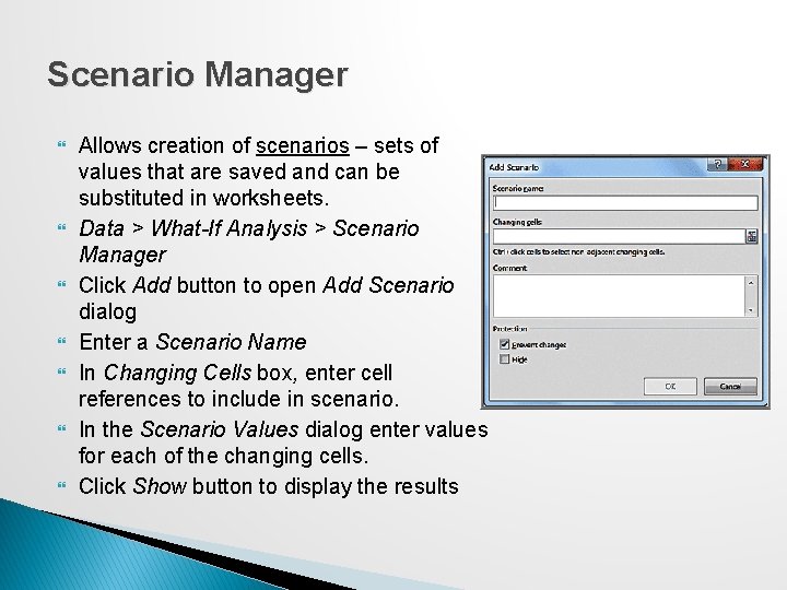
Scenario Manager Allows creation of scenarios – sets of values that are saved and can be substituted in worksheets. Data > What-If Analysis > Scenario Manager Click Add button to open Add Scenario dialog Enter a Scenario Name In Changing Cells box, enter cell references to include in scenario. In the Scenario Values dialog enter values for each of the changing cells. Click Show button to display the results

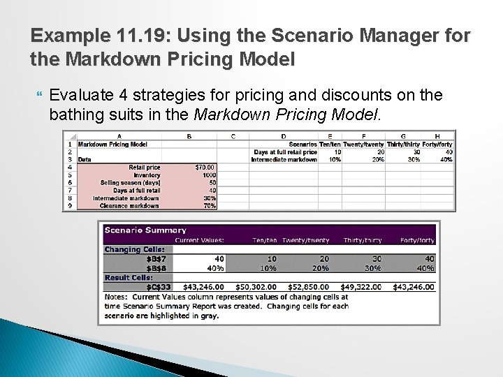
Example 11. 19: Using the Scenario Manager for the Markdown Pricing Model Evaluate 4 strategies for pricing and discounts on the bathing suits in the Markdown Pricing Model.

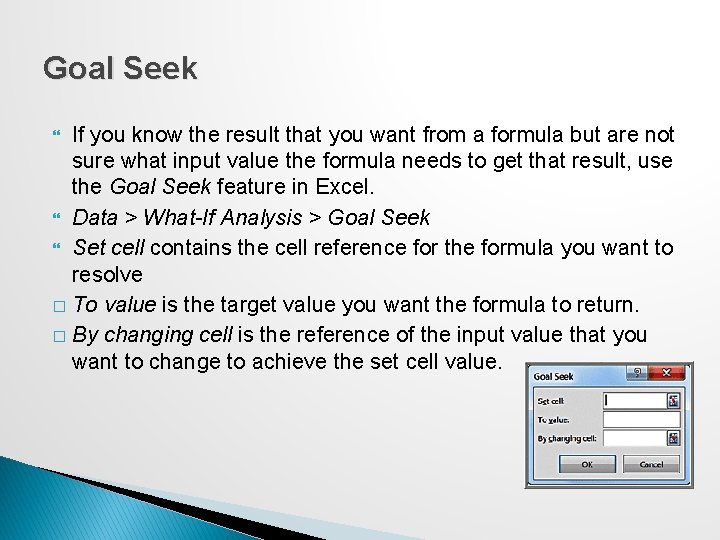
Goal Seek If you know the result that you want from a formula but are not sure what input value the formula needs to get that result, use the Goal Seek feature in Excel. Data > What-If Analysis > Goal Seek Set cell contains the cell reference for the formula you want to resolve � To value is the target value you want the formula to return. � By changing cell is the reference of the input value that you want to change to achieve the set cell value.

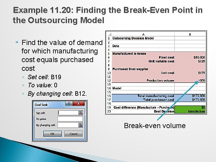
Example 11. 20: Finding the Break-Even Point in the Outsourcing Model Find the value of demand for which manufacturing cost equals purchased cost ◦ Set cell: B 19 ◦ To value: 0 ◦ By changing cell: B 12. Break-even volume

Parametric Sensitivity Analysis Using Analytic Solver Platform Parametric sensitivity analysis is the term used by Analytic Solver Platform for systematic methods of what-if analysis. ◦ A parameter is simply a piece of input data in a model. You can create data tables and tornado charts.

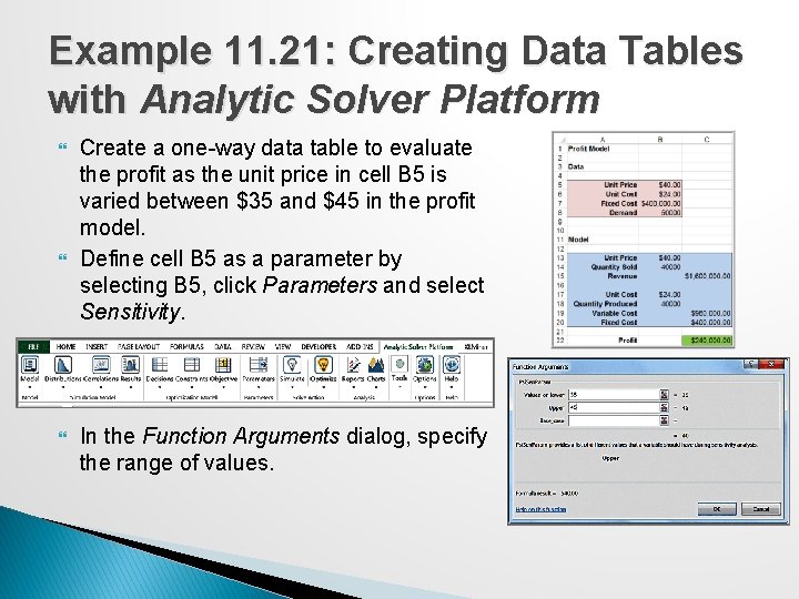
Example 11. 21: Creating Data Tables with Analytic Solver Platform Create a one-way data table to evaluate the profit as the unit price in cell B 5 is varied between $35 and $45 in the profit model. Define cell B 5 as a parameter by selecting B 5, click Parameters and select Sensitivity. In the Function Arguments dialog, specify the range of values.

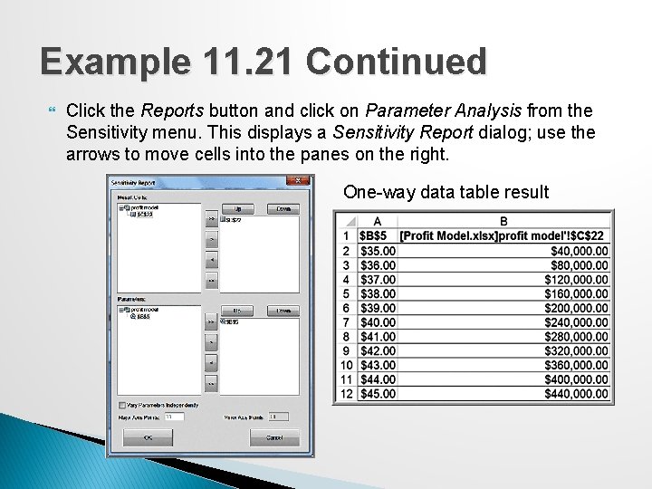
Example 11. 21 Continued Click the Reports button and click on Parameter Analysis from the Sensitivity menu. This displays a Sensitivity Report dialog; use the arrows to move cells into the panes on the right. One-way data table result

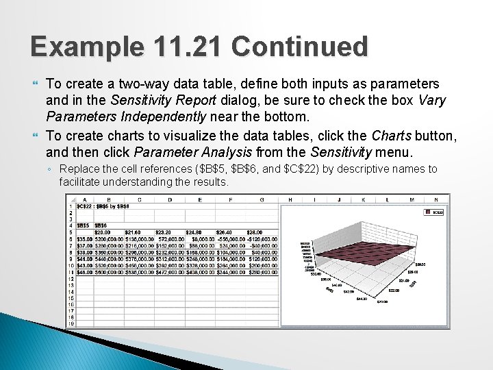
Example 11. 21 Continued To create a two-way data table, define both inputs as parameters and in the Sensitivity Report dialog, be sure to check the box Vary Parameters Independently near the bottom. To create charts to visualize the data tables, click the Charts button, and then click Parameter Analysis from the Sensitivity menu. ◦ Replace the cell references ($B$5, $B$6, and $C$22) by descriptive names to facilitate understanding the results.

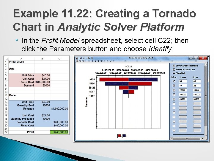
Tornado Charts A tornado chart shows the impact that variation in a model input has on some output while holding all other inputs constant. ◦ Shows which inputs are the least and most influential on the output. ◦ Helps you select the inputs that you would want to further analyze. Analytic Solver Platform automatically identifies all the data input cells on which the output cell depends and creates the chart.

Example 11. 22: Creating a Tornado Chart in Analytic Solver Platform In the Profit Model spreadsheet, select cell C 22; then click the Parameters button and choose Identify.