Chapter 11 Response Surface Methods and Other Approaches

Chapter 11 Response Surface Methods and Other Approaches to Process Optimization 1

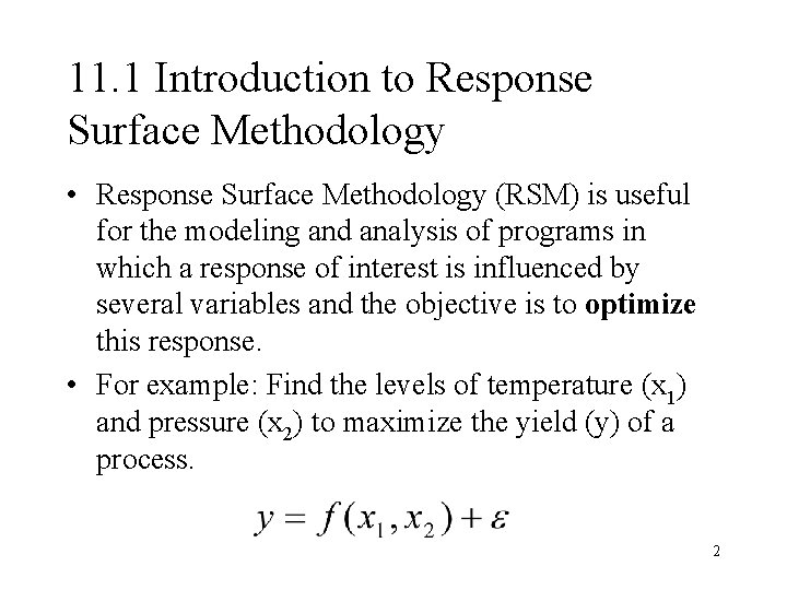
11. 1 Introduction to Response Surface Methodology • Response Surface Methodology (RSM) is useful for the modeling and analysis of programs in which a response of interest is influenced by several variables and the objective is to optimize this response. • For example: Find the levels of temperature (x 1) and pressure (x 2) to maximize the yield (y) of a process. 2

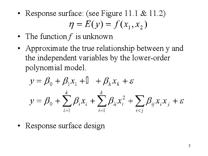
• Response surface: (see Figure 11. 1 & 11. 2) • The function f is unknown • Approximate the true relationship between y and the independent variables by the lower-order polynomial model. • Response surface design 3

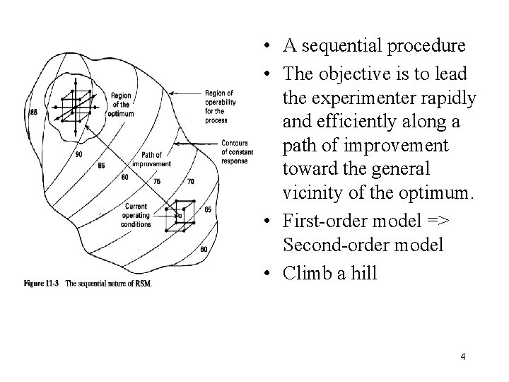
• A sequential procedure • The objective is to lead the experimenter rapidly and efficiently along a path of improvement toward the general vicinity of the optimum. • First-order model => Second-order model • Climb a hill 4

11. 2 The Method of Steepest Ascent • Assume that the first-order model is an adequate approximation to the true surface in a small ragion of the x’s. • The method of steepest ascent: A procedure for moving sequentially along the path of steepest ascent. 5

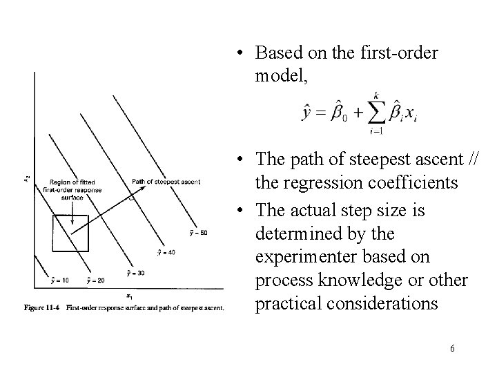
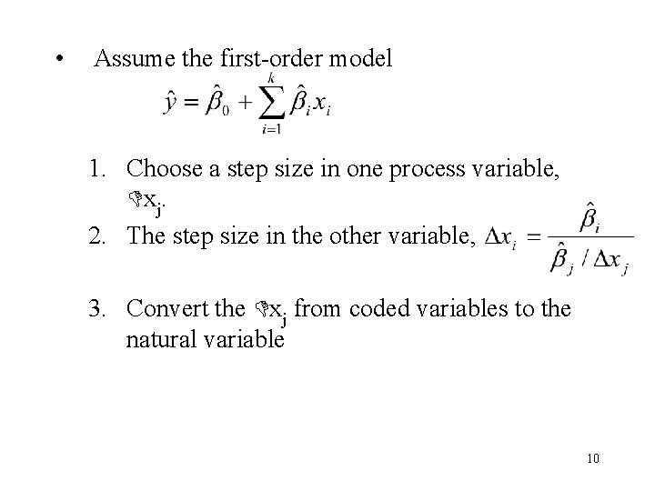
• Based on the first-order model, • The path of steepest ascent // the regression coefficients • The actual step size is determined by the experimenter based on process knowledge or other practical considerations 6

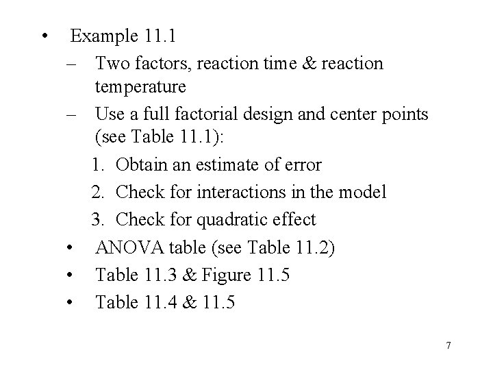
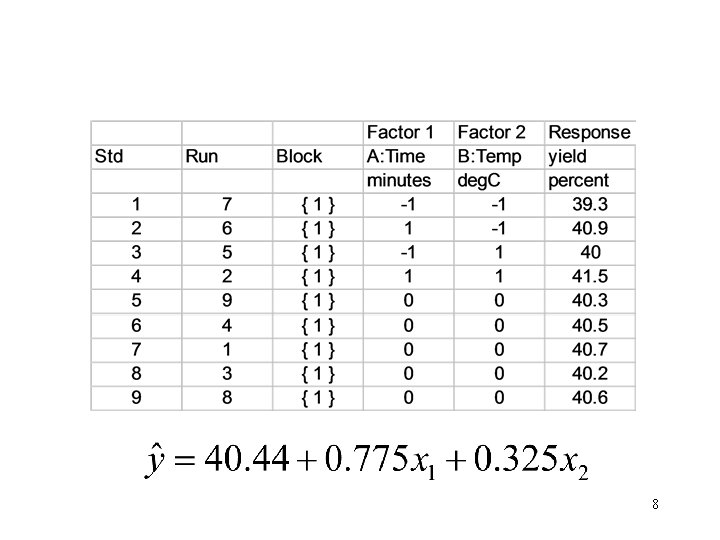
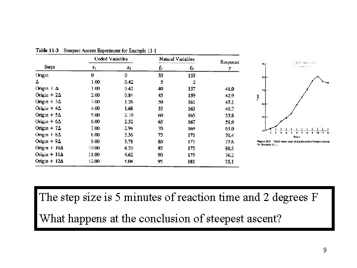
• Example 11. 1 – Two factors, reaction time & reaction temperature – Use a full factorial design and center points (see Table 11. 1): 1. Obtain an estimate of error 2. Check for interactions in the model 3. Check for quadratic effect • ANOVA table (see Table 11. 2) • Table 11. 3 & Figure 11. 5 • Table 11. 4 & 11. 5 7

8

The step size is 5 minutes of reaction time and 2 degrees F What happens at the conclusion of steepest ascent? 9

• Assume the first-order model 1. Choose a step size in one process variable, xj. 2. The step size in the other variable, 3. Convert the xj from coded variables to the natural variable 10

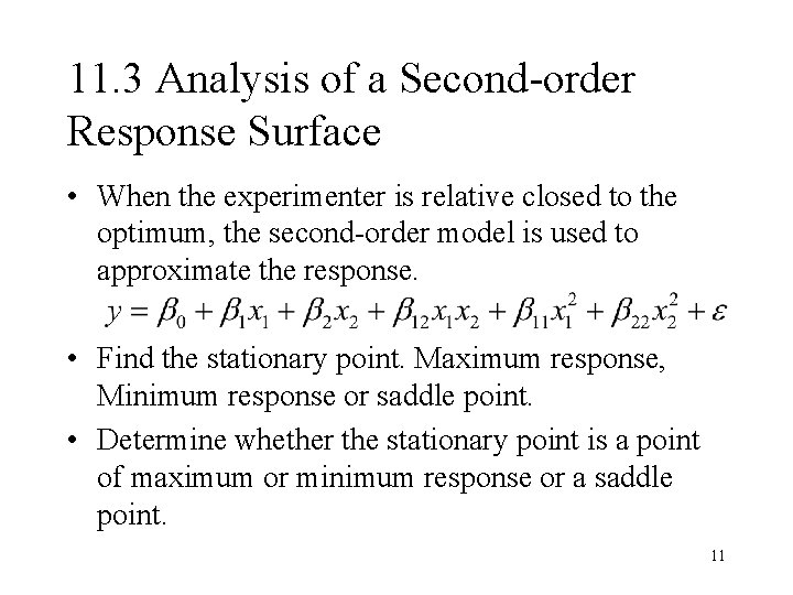
11. 3 Analysis of a Second-order Response Surface • When the experimenter is relative closed to the optimum, the second-order model is used to approximate the response. • Find the stationary point. Maximum response, Minimum response or saddle point. • Determine whether the stationary point is a point of maximum or minimum response or a saddle point. 11

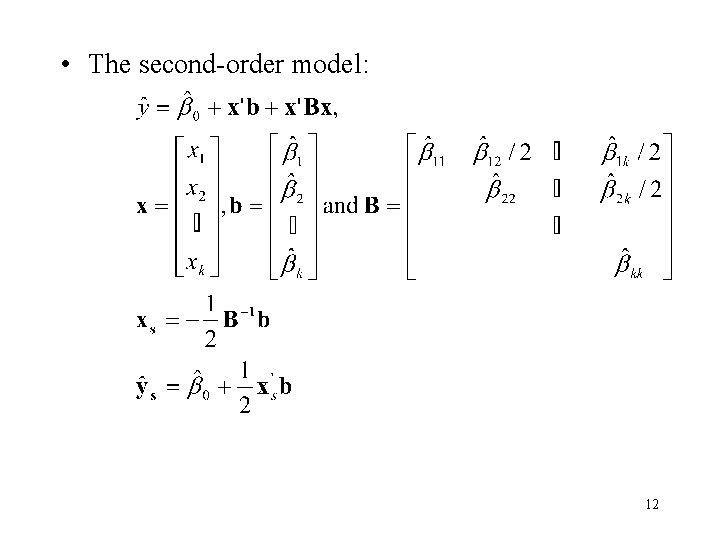
• The second-order model: 12

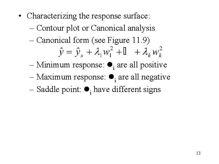
• Characterizing the response surface: – Contour plot or Canonical analysis – Canonical form (see Figure 11. 9) – Minimum response: i are all positive – Maximum response: i are all negative – Saddle point: i have different signs 13

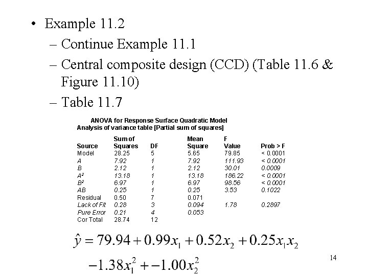
• Example 11. 2 – Continue Example 11. 1 – Central composite design (CCD) (Table 11. 6 & Figure 11. 10) – Table 11. 7 ANOVA for Response Surface Quadratic Model Analysis of variance table [Partial sum of squares] Source Model A B A 2 B 2 AB Residual Lack of Fit Pure Error Cor Total Sum of Squares 28. 25 7. 92 2. 12 13. 18 6. 97 0. 25 0. 50 0. 28 0. 21 28. 74 DF 5 1 1 1 7 3 4 12 Mean Square 5. 65 7. 92 2. 12 13. 18 6. 97 0. 25 0. 071 0. 094 0. 053 F Value 79. 85 111. 93 30. 01 186. 22 98. 56 3. 53 Prob > F < 0. 0001 0. 0009 < 0. 0001 0. 1022 1. 78 0. 2897 14

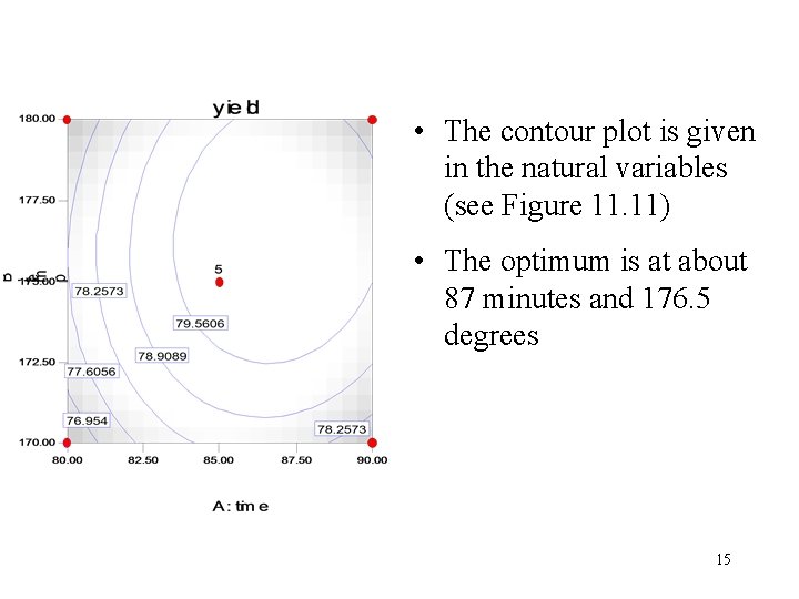
• The contour plot is given in the natural variables (see Figure 11. 11) • The optimum is at about 87 minutes and 176. 5 degrees 15

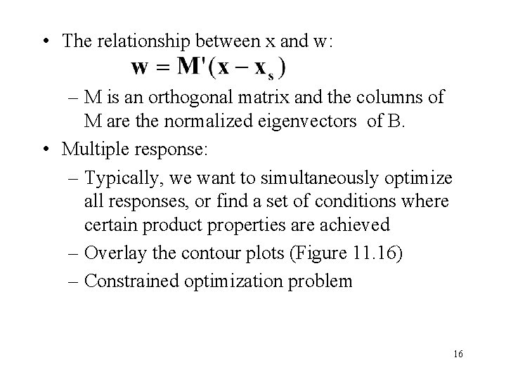
• The relationship between x and w: – M is an orthogonal matrix and the columns of M are the normalized eigenvectors of B. • Multiple response: – Typically, we want to simultaneously optimize all responses, or find a set of conditions where certain product properties are achieved – Overlay the contour plots (Figure 11. 16) – Constrained optimization problem 16

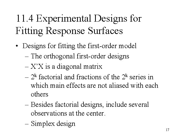
11. 4 Experimental Designs for Fitting Response Surfaces • Designs for fitting the first-order model – The orthogonal first-order designs – X’X is a diagonal matrix – 2 k factorial and fractions of the 2 k series in which main effects are not aliased with each others – Besides factorial designs, include several observations at the center. – Simplex design 17

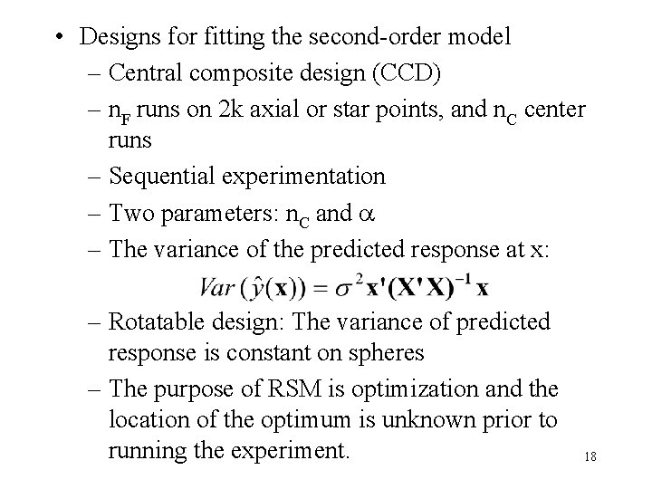
• Designs for fitting the second-order model – Central composite design (CCD) – n. F runs on 2 k axial or star points, and n. C center runs – Sequential experimentation – Two parameters: n. C and – The variance of the predicted response at x: – Rotatable design: The variance of predicted response is constant on spheres – The purpose of RSM is optimization and the location of the optimum is unknown prior to running the experiment. 18

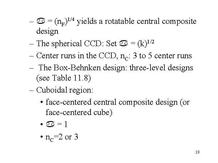
– = (n. F)1/4 yields a rotatable central composite design – The spherical CCD: Set = (k)1/2 – Center runs in the CCD, n. C: 3 to 5 center runs – The Box-Behnken design: three-level designs (see Table 11. 8) – Cuboidal region: • face-centered central composite design (or face-centered cube) • =1 • n. C=2 or 3 19