Chapter 11 Optimal Portfolio Choice and the Capital

Chapter 11 Optimal Portfolio Choice and the Capital Asset Pricing Model

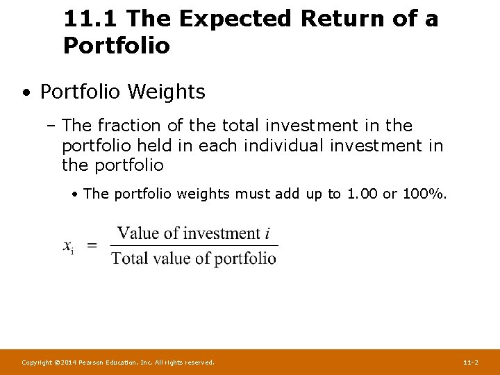
11. 1 The Expected Return of a Portfolio • Portfolio Weights – The fraction of the total investment in the portfolio held in each individual investment in the portfolio • The portfolio weights must add up to 1. 00 or 100%. Copyright © 2014 Pearson Education, Inc. All rights reserved. 11 -2

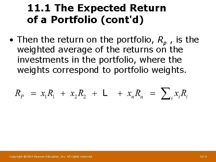
11. 1 The Expected Return of a Portfolio (cont'd) • Then the return on the portfolio, Rp , is the weighted average of the returns on the investments in the portfolio, where the weights correspond to portfolio weights. Copyright © 2014 Pearson Education, Inc. All rights reserved. 11 -3

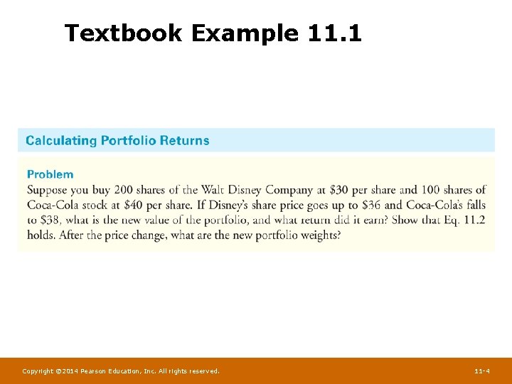
Textbook Example 11. 1 Copyright © 2014 Pearson Education, Inc. All rights reserved. 11 -4

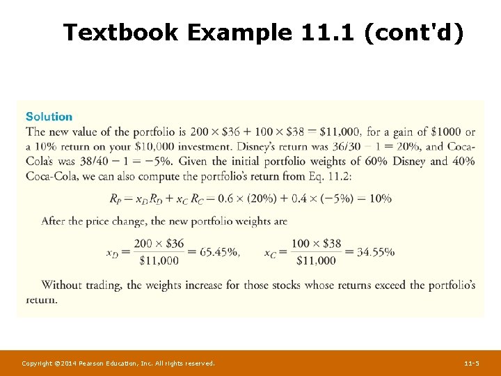
Textbook Example 11. 1 (cont'd) Copyright © 2014 Pearson Education, Inc. All rights reserved. 11 -5

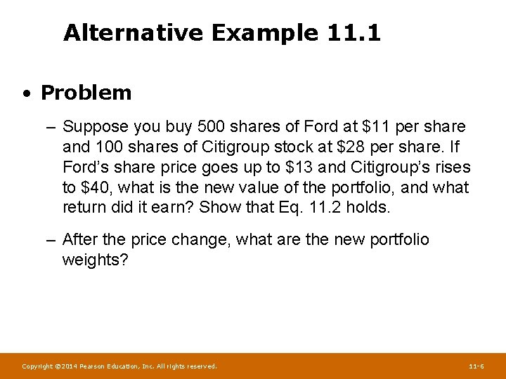
Alternative Example 11. 1 • Problem – Suppose you buy 500 shares of Ford at $11 per share and 100 shares of Citigroup stock at $28 per share. If Ford’s share price goes up to $13 and Citigroup’s rises to $40, what is the new value of the portfolio, and what return did it earn? Show that Eq. 11. 2 holds. – After the price change, what are the new portfolio weights? Copyright © 2014 Pearson Education, Inc. All rights reserved. 11 -6

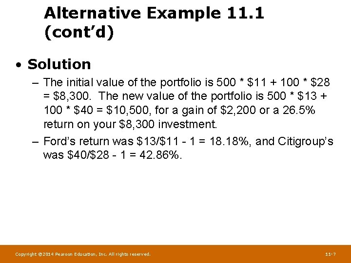
Alternative Example 11. 1 (cont’d) • Solution – The initial value of the portfolio is 500 * $11 + 100 * $28 = $8, 300. The new value of the portfolio is 500 * $13 + 100 * $40 = $10, 500, for a gain of $2, 200 or a 26. 5% return on your $8, 300 investment. – Ford’s return was $13/$11 - 1 = 18. 18%, and Citigroup’s was $40/$28 - 1 = 42. 86%. Copyright © 2014 Pearson Education, Inc. All rights reserved. 11 -7

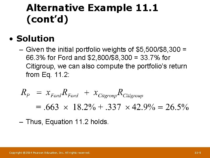
Alternative Example 11. 1 (cont’d) • Solution – Given the initial portfolio weights of $5, 500/$8, 300 = 66. 3% for Ford and $2, 800/$8, 300 = 33. 7% for Citigroup, we can also compute the portfolio’s return from Eq. 11. 2: – Thus, Equation 11. 2 holds. Copyright © 2014 Pearson Education, Inc. All rights reserved. 11 -8

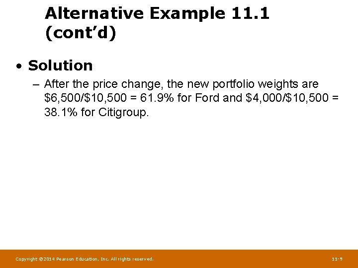
Alternative Example 11. 1 (cont’d) • Solution – After the price change, the new portfolio weights are $6, 500/$10, 500 = 61. 9% for Ford and $4, 000/$10, 500 = 38. 1% for Citigroup. Copyright © 2014 Pearson Education, Inc. All rights reserved. 11 -9

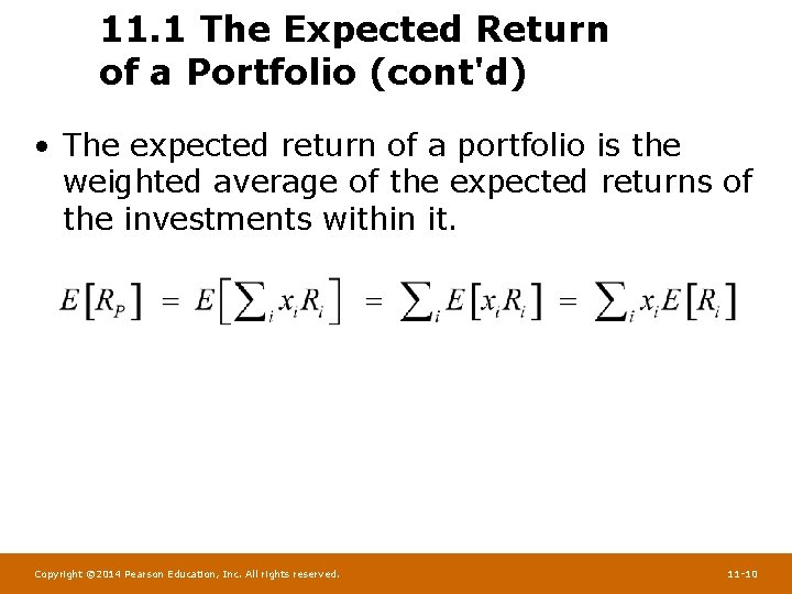
11. 1 The Expected Return of a Portfolio (cont'd) • The expected return of a portfolio is the weighted average of the expected returns of the investments within it. Copyright © 2014 Pearson Education, Inc. All rights reserved. 11 -10

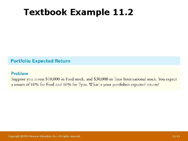
Textbook Example 11. 2 Copyright © 2014 Pearson Education, Inc. All rights reserved. 11 -11

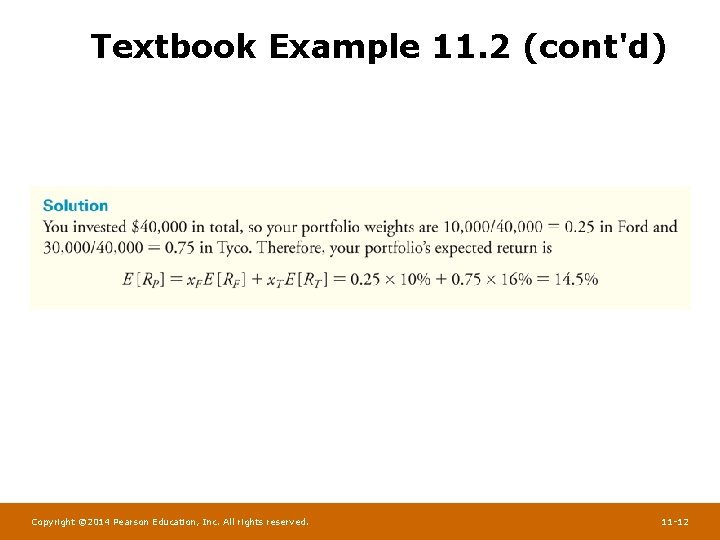
Textbook Example 11. 2 (cont'd) Copyright © 2014 Pearson Education, Inc. All rights reserved. 11 -12

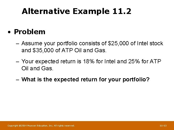
Alternative Example 11. 2 • Problem – Assume your portfolio consists of $25, 000 of Intel stock and $35, 000 of ATP Oil and Gas. – Your expected return is 18% for Intel and 25% for ATP Oil and Gas. – What is the expected return for your portfolio? Copyright © 2014 Pearson Education, Inc. All rights reserved. 11 -13

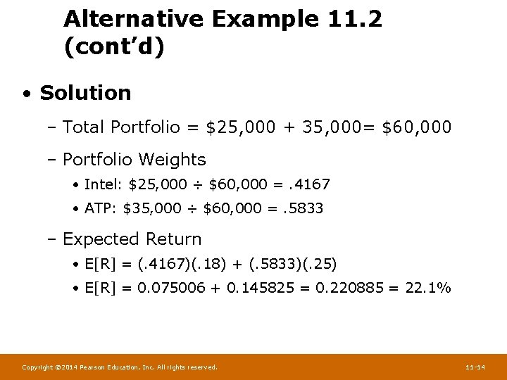
Alternative Example 11. 2 (cont’d) • Solution – Total Portfolio = $25, 000 + 35, 000= $60, 000 – Portfolio Weights • Intel: $25, 000 ÷ $60, 000 =. 4167 • ATP: $35, 000 ÷ $60, 000 =. 5833 – Expected Return • E[R] = (. 4167)(. 18) + (. 5833)(. 25) • E[R] = 0. 075006 + 0. 145825 = 0. 220885 = 22. 1% Copyright © 2014 Pearson Education, Inc. All rights reserved. 11 -14

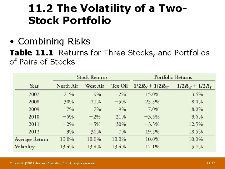
11. 2 The Volatility of a Two. Stock Portfolio • Combining Risks Table 11. 1 Returns for Three Stocks, and Portfolios of Pairs of Stocks Copyright © 2014 Pearson Education, Inc. All rights reserved. 11 -15

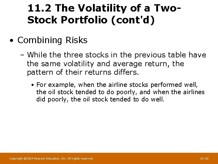
11. 2 The Volatility of a Two. Stock Portfolio (cont'd) • Combining Risks – While three stocks in the previous table have the same volatility and average return, the pattern of their returns differs. • For example, when the airline stocks performed well, the oil stock tended to do poorly, and when the airlines did poorly, the oil stock tended to do well. Copyright © 2014 Pearson Education, Inc. All rights reserved. 11 -16

11. 2 The Volatility of a Two. Stock Portfolio (cont'd) • Combining Risks – Consider the portfolio which consists of equal investments in West Air and Tex Oil. The average return of the portfolio is equal to the average return of the two stocks – However, the volatility of 5. 1% is much less than the volatility of the two individual stocks. Copyright © 2014 Pearson Education, Inc. All rights reserved. 11 -17

11. 2 The Volatility of a Two. Stock Portfolio (cont'd) • Combining Risks – By combining stocks into a portfolio, we reduce risk through diversification. – The amount of risk that is eliminated in a portfolio depends on the degree to which the stocks face common risks and their prices move together. Copyright © 2014 Pearson Education, Inc. All rights reserved. 11 -18

Determining Covariance and Correlation • To find the risk of a portfolio, one must know the degree to which the stocks’ returns move together. Copyright © 2014 Pearson Education, Inc. All rights reserved. 11 -19

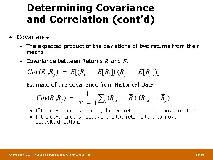
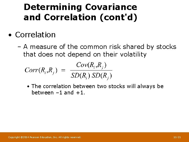
Determining Covariance and Correlation (cont'd) • Covariance – The expected product of the deviations of two returns from their means – Covariance between Returns Ri and Rj – Estimate of the Covariance from Historical Data • If the covariance is positive, the two returns tend to move together. • If the covariance is negative, the two returns tend to move in opposite directions. Copyright © 2014 Pearson Education, Inc. All rights reserved. 11 -20

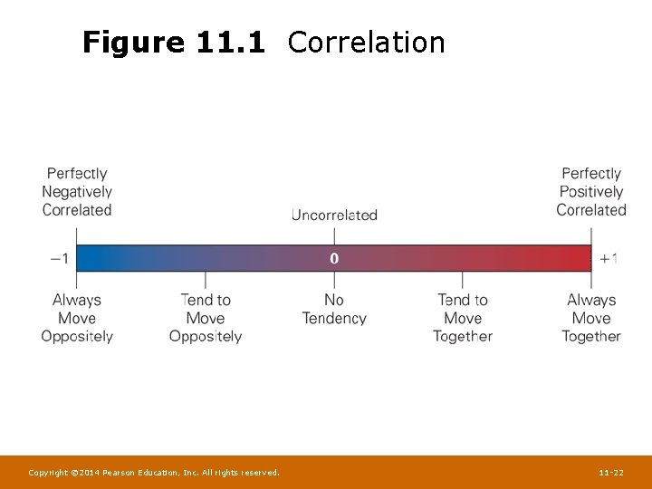
Determining Covariance and Correlation (cont'd) • Correlation – A measure of the common risk shared by stocks that does not depend on their volatility • The correlation between two stocks will always be between – 1 and +1. Copyright © 2014 Pearson Education, Inc. All rights reserved. 11 -21

Figure 11. 1 Correlation Copyright © 2014 Pearson Education, Inc. All rights reserved. 11 -22

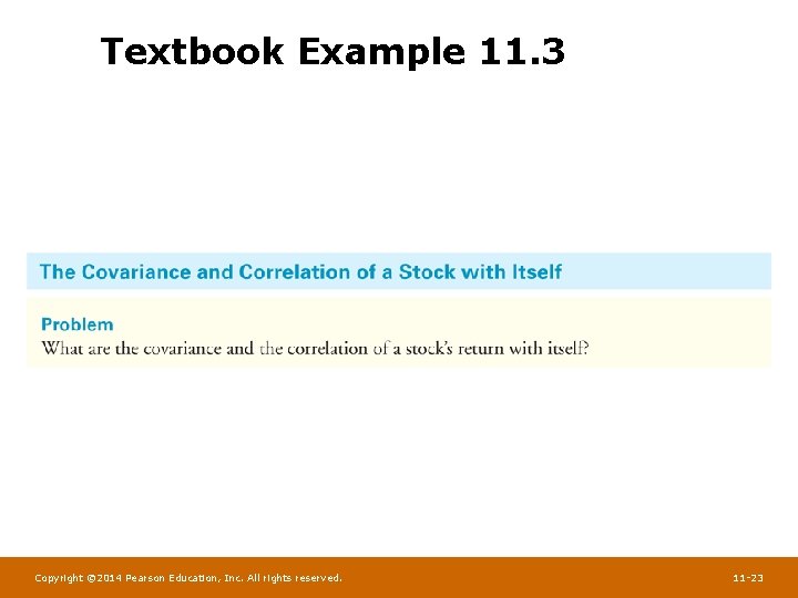
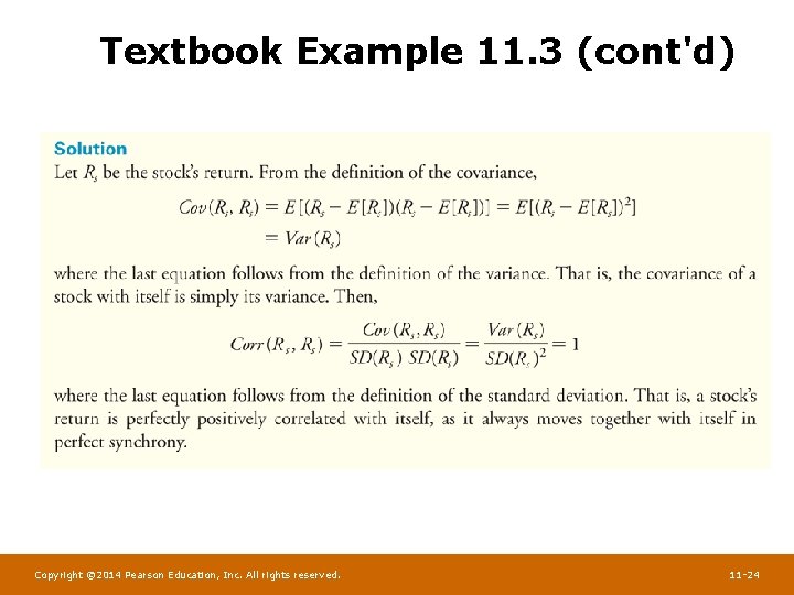
Textbook Example 11. 3 Copyright © 2014 Pearson Education, Inc. All rights reserved. 11 -23

Textbook Example 11. 3 (cont'd) Copyright © 2014 Pearson Education, Inc. All rights reserved. 11 -24

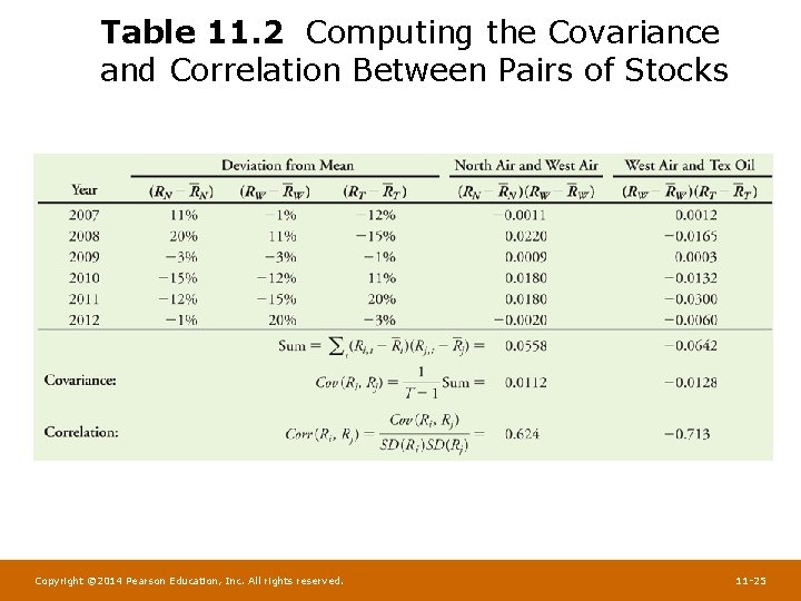
Table 11. 2 Computing the Covariance and Correlation Between Pairs of Stocks Copyright © 2014 Pearson Education, Inc. All rights reserved. 11 -25

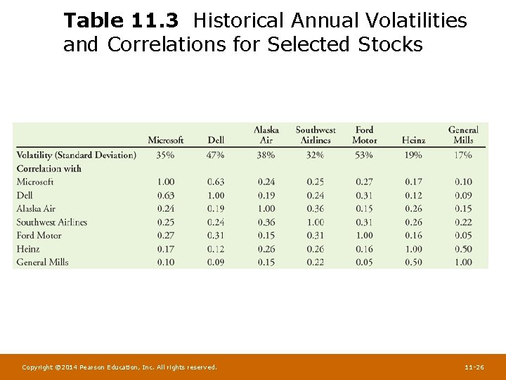
Table 11. 3 Historical Annual Volatilities and Correlations for Selected Stocks Copyright © 2014 Pearson Education, Inc. All rights reserved. 11 -26

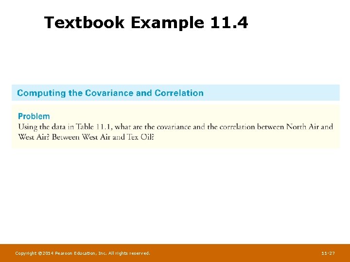
Textbook Example 11. 4 Copyright © 2014 Pearson Education, Inc. All rights reserved. 11 -27

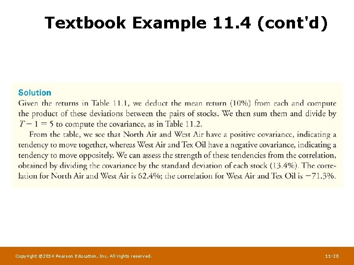
Textbook Example 11. 4 (cont'd) Copyright © 2014 Pearson Education, Inc. All rights reserved. 11 -28

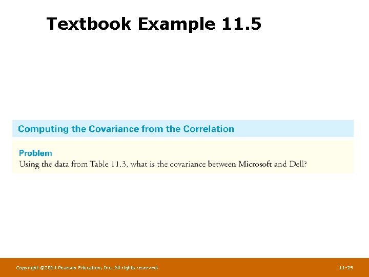
Textbook Example 11. 5 Copyright © 2014 Pearson Education, Inc. All rights reserved. 11 -29

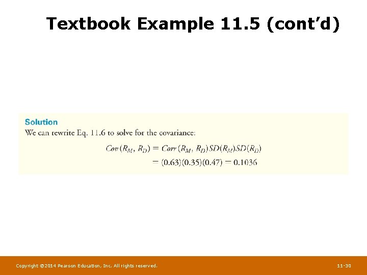
Textbook Example 11. 5 (cont’d) Copyright © 2014 Pearson Education, Inc. All rights reserved. 11 -30

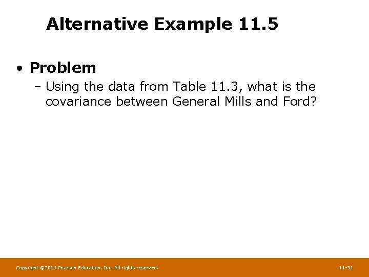
Alternative Example 11. 5 • Problem – Using the data from Table 11. 3, what is the covariance between General Mills and Ford? Copyright © 2014 Pearson Education, Inc. All rights reserved. 11 -31

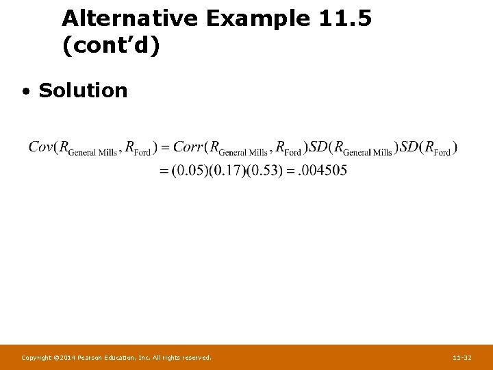
Alternative Example 11. 5 (cont’d) • Solution Copyright © 2014 Pearson Education, Inc. All rights reserved. 11 -32

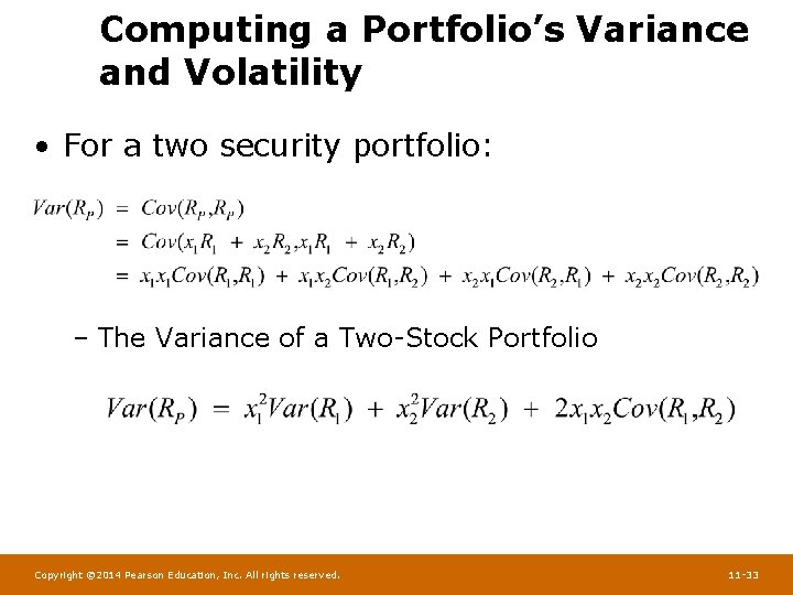
Computing a Portfolio’s Variance and Volatility • For a two security portfolio: – The Variance of a Two-Stock Portfolio Copyright © 2014 Pearson Education, Inc. All rights reserved. 11 -33

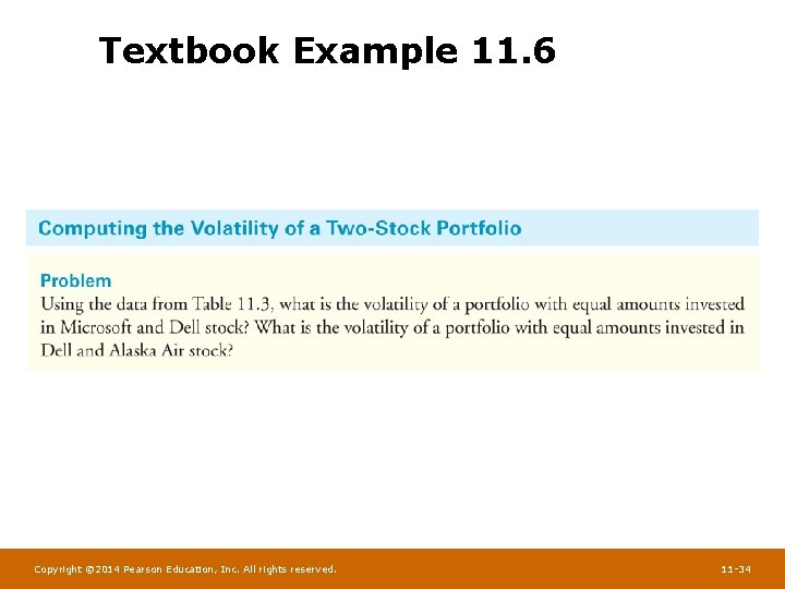
Textbook Example 11. 6 Copyright © 2014 Pearson Education, Inc. All rights reserved. 11 -34

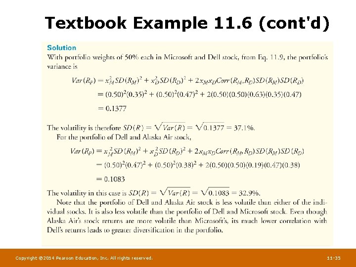
Textbook Example 11. 6 (cont'd) Copyright © 2014 Pearson Education, Inc. All rights reserved. 11 -35

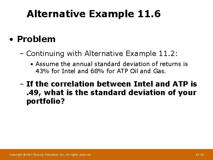
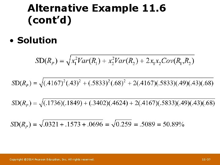
Alternative Example 11. 6 • Problem – Continuing with Alternative Example 11. 2: • Assume the annual standard deviation of returns is 43% for Intel and 68% for ATP Oil and Gas. – If the correlation between Intel and ATP is. 49, what is the standard deviation of your portfolio? Copyright © 2014 Pearson Education, Inc. All rights reserved. 11 -36

Alternative Example 11. 6 (cont’d) • Solution Copyright © 2014 Pearson Education, Inc. All rights reserved. 11 -37

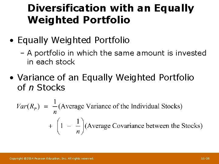
Diversification with an Equally Weighted Portfolio • Equally Weighted Portfolio – A portfolio in which the same amount is invested in each stock • Variance of an Equally Weighted Portfolio of n Stocks Copyright © 2014 Pearson Education, Inc. All rights reserved. 11 -38

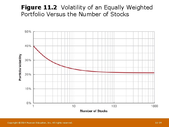
Figure 11. 2 Volatility of an Equally Weighted Portfolio Versus the Number of Stocks Copyright © 2014 Pearson Education, Inc. All rights reserved. 11 -39

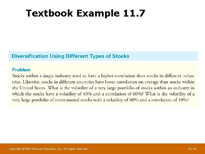
Textbook Example 11. 7 Copyright © 2014 Pearson Education, Inc. All rights reserved. 11 -40

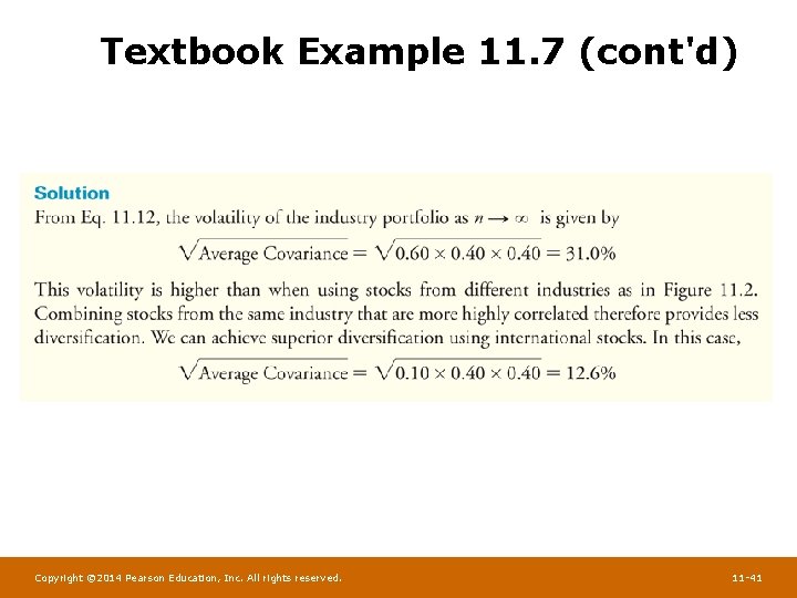
Textbook Example 11. 7 (cont'd) Copyright © 2014 Pearson Education, Inc. All rights reserved. 11 -41

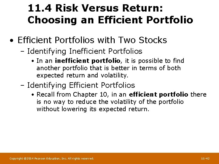
11. 4 Risk Versus Return: Choosing an Efficient Portfolio • Efficient Portfolios with Two Stocks – Identifying Inefficient Portfolios • In an inefficient portfolio, it is possible to find another portfolio that is better in terms of both expected return and volatility. – Identifying Efficient Portfolios • Recall from Chapter 10, in an efficient portfolio there is no way to reduce the volatility of the portfolio without lowering its expected return. Copyright © 2014 Pearson Education, Inc. All rights reserved. 11 -42

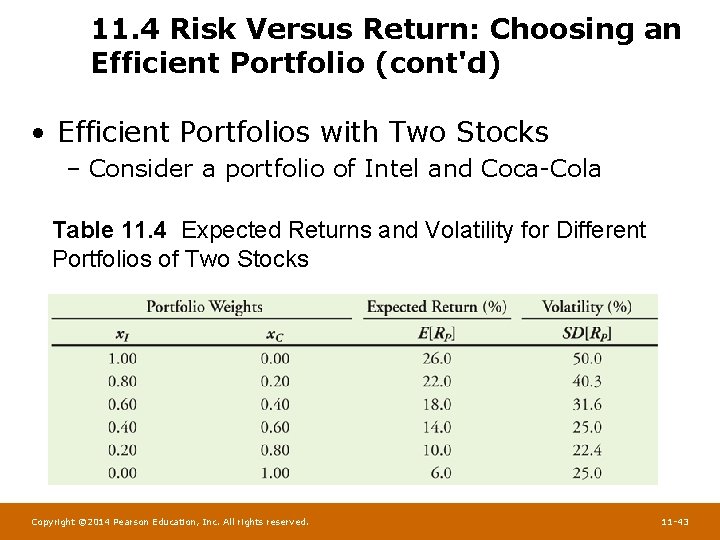
11. 4 Risk Versus Return: Choosing an Efficient Portfolio (cont'd) • Efficient Portfolios with Two Stocks – Consider a portfolio of Intel and Coca-Cola Table 11. 4 Expected Returns and Volatility for Different Portfolios of Two Stocks Copyright © 2014 Pearson Education, Inc. All rights reserved. 11 -43

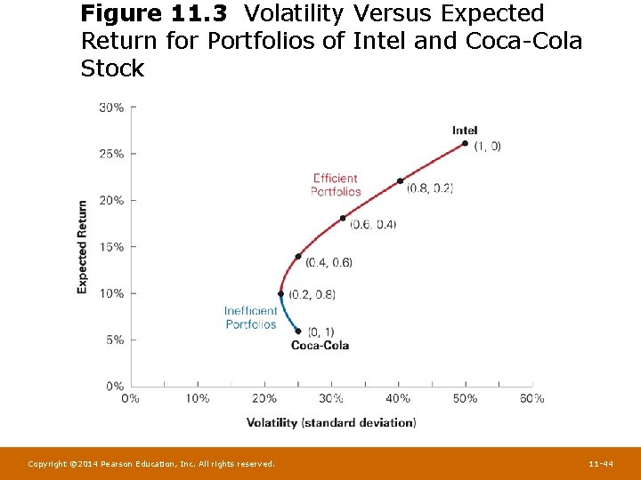
Figure 11. 3 Volatility Versus Expected Return for Portfolios of Intel and Coca-Cola Stock Copyright © 2014 Pearson Education, Inc. All rights reserved. 11 -44

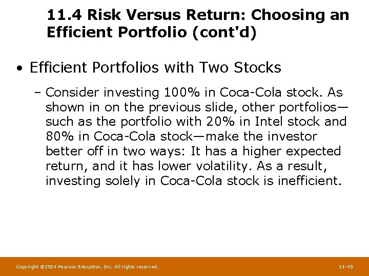
11. 4 Risk Versus Return: Choosing an Efficient Portfolio (cont'd) • Efficient Portfolios with Two Stocks – Consider investing 100% in Coca-Cola stock. As shown in on the previous slide, other portfolios— such as the portfolio with 20% in Intel stock and 80% in Coca-Cola stock—make the investor better off in two ways: It has a higher expected return, and it has lower volatility. As a result, investing solely in Coca-Cola stock is inefficient. Copyright © 2014 Pearson Education, Inc. All rights reserved. 11 -45

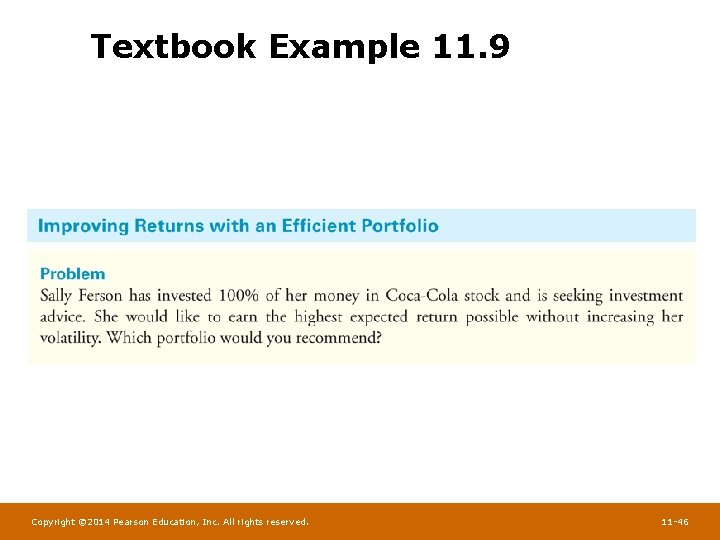
Textbook Example 11. 9 Copyright © 2014 Pearson Education, Inc. All rights reserved. 11 -46

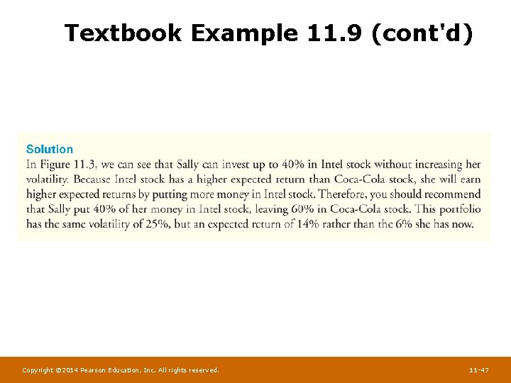
Textbook Example 11. 9 (cont'd) Copyright © 2014 Pearson Education, Inc. All rights reserved. 11 -47

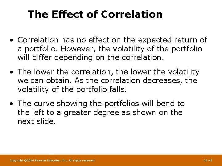
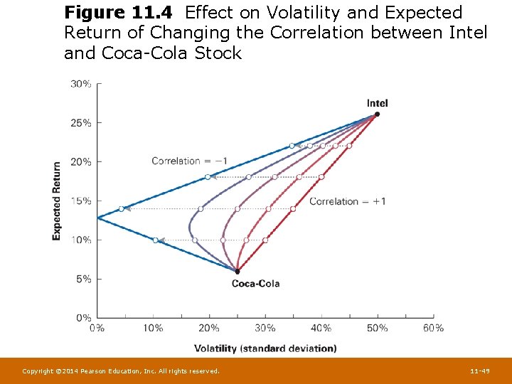
The Effect of Correlation • Correlation has no effect on the expected return of a portfolio. However, the volatility of the portfolio will differ depending on the correlation. • The lower the correlation, the lower the volatility we can obtain. As the correlation decreases, the volatility of the portfolio falls. • The curve showing the portfolios will bend to the left to a greater degree as shown on the next slide. Copyright © 2014 Pearson Education, Inc. All rights reserved. 11 -48

Figure 11. 4 Effect on Volatility and Expected Return of Changing the Correlation between Intel and Coca-Cola Stock Copyright © 2014 Pearson Education, Inc. All rights reserved. 11 -49

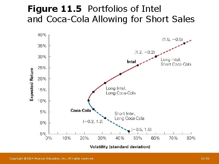
Short Sales • Long Position – A positive investment in a security • Short Position – A negative investment in a security – In a short sale, you sell a stock that you do not own and then buy that stock back in the future. – Short selling is an advantageous strategy if you expect a stock price to decline in the future. Copyright © 2014 Pearson Education, Inc. All rights reserved. 11 -50

Figure 11. 5 Portfolios of Intel and Coca-Cola Allowing for Short Sales Copyright © 2014 Pearson Education, Inc. All rights reserved. 11 -51

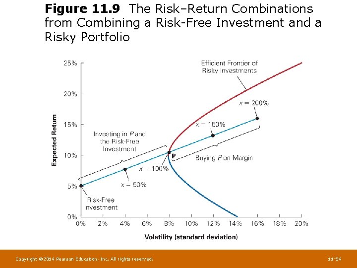
11. 5 Risk-Free Saving and Borrowing • Risk can also be reduced by investing a portion of a portfolio in a risk-free investment, like T-Bills. However, doing so will likely reduce the expected return. • On the other hand, an aggressive investor who is seeking high expected returns might decide to borrow money to invest even more in the stock market. Copyright © 2014 Pearson Education, Inc. All rights reserved. 11 -52

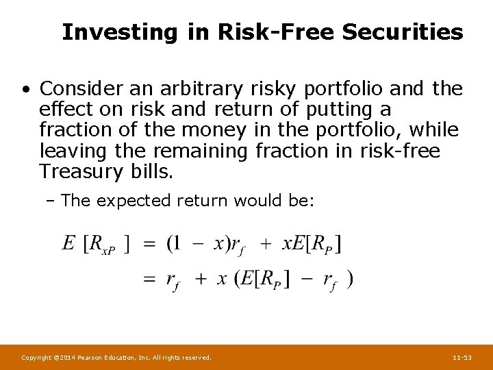
Investing in Risk-Free Securities • Consider an arbitrary risky portfolio and the effect on risk and return of putting a fraction of the money in the portfolio, while leaving the remaining fraction in risk-free Treasury bills. – The expected return would be: Copyright © 2014 Pearson Education, Inc. All rights reserved. 11 -53

Figure 11. 9 The Risk–Return Combinations from Combining a Risk-Free Investment and a Risky Portfolio Copyright © 2014 Pearson Education, Inc. All rights reserved. 11 -54

Borrowing and Buying Stocks on Margin • Buying Stocks on Margin – Borrowing money to invest in a stock. – A portfolio that consists of a short position in the risk-free investment is known as a levered portfolio. Margin investing is a risky investment strategy. Copyright © 2014 Pearson Education, Inc. All rights reserved. 11 -55

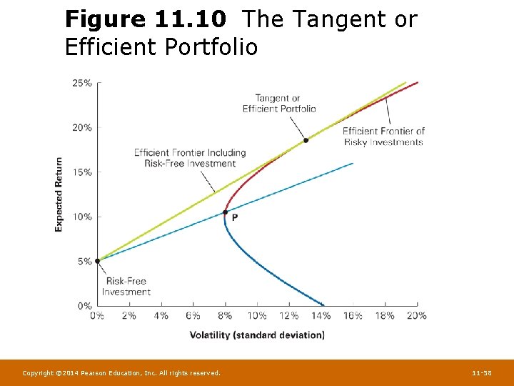
Identifying the Tangent Portfolio • To earn the highest possible expected return for any level of volatility we must find the portfolio that generates the steepest possible line when combined with the risk-free investment. Copyright © 2014 Pearson Education, Inc. All rights reserved. 11 -56

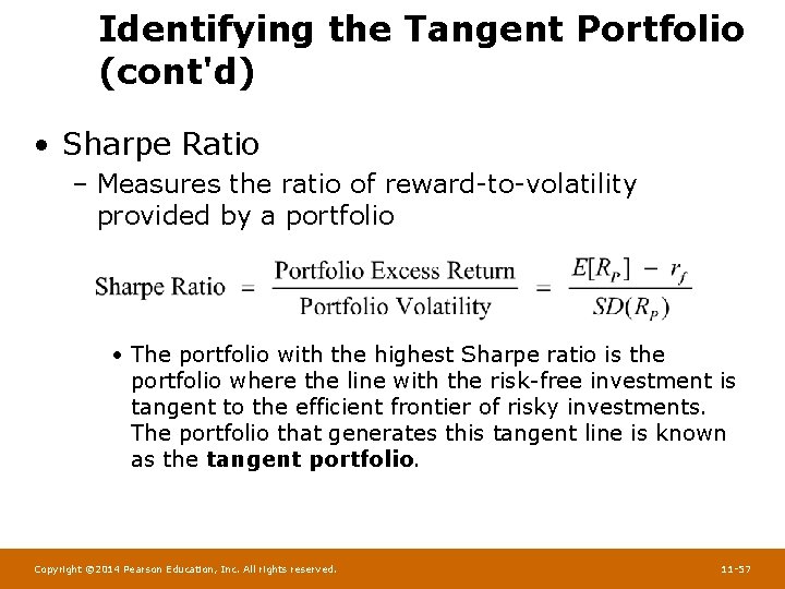
Identifying the Tangent Portfolio (cont'd) • Sharpe Ratio – Measures the ratio of reward-to-volatility provided by a portfolio • The portfolio with the highest Sharpe ratio is the portfolio where the line with the risk-free investment is tangent to the efficient frontier of risky investments. The portfolio that generates this tangent line is known as the tangent portfolio. Copyright © 2014 Pearson Education, Inc. All rights reserved. 11 -57

Figure 11. 10 The Tangent or Efficient Portfolio Copyright © 2014 Pearson Education, Inc. All rights reserved. 11 -58

Identifying the Tangent Portfolio (cont'd) • Combinations of the risk-free asset and the tangent portfolio provide the best risk and return tradeoff available to an investor. – This means that the tangent portfolio is efficient and that all efficient portfolios are combinations of the risk-free investment and the tangent portfolio. Every investor should invest in the tangent portfolio independent of his or her taste for risk. Copyright © 2014 Pearson Education, Inc. All rights reserved. 11 -59

Identifying the Tangent Portfolio (cont'd) • An investor’s preferences will determine only how much to invest in the tangent portfolio versus the risk-free investment. – Conservative investors will invest a small amount in the tangent portfolio. – Aggressive investors will invest more in the tangent portfolio. – Both types of investors will choose to hold the same portfolio of risky assets, the tangent portfolio, which is the efficient portfolio. Copyright © 2014 Pearson Education, Inc. All rights reserved. 11 -60

11. 6 The Efficient Portfolio and Required Returns • Portfolio Improvement: Beta and the Required Return – Assume there is a portfolio of risky securities, P. To determine whether P has the highest possible Sharpe ratio, consider whether its Sharpe ratio could be raised by adding more of some investment i to the portfolio. – The contribution of investment i to the volatility of the portfolio depends on the risk that i has in common with the portfolio, which is measured by i’s volatility multiplied by its correlation with P. Copyright © 2014 Pearson Education, Inc. All rights reserved. 11 -61

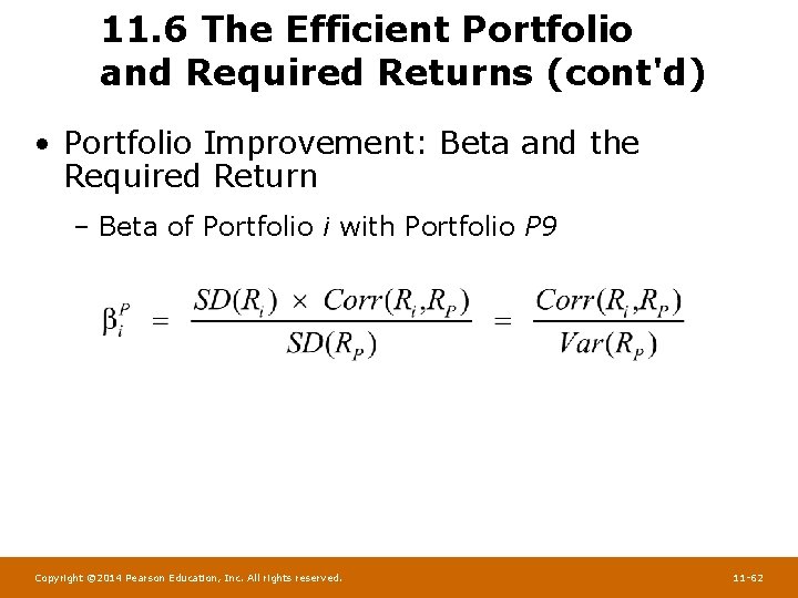
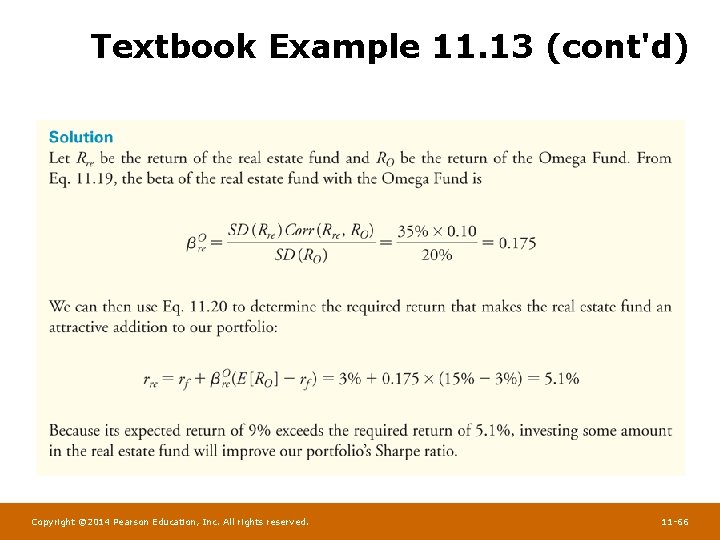
11. 6 The Efficient Portfolio and Required Returns (cont'd) • Portfolio Improvement: Beta and the Required Return – Beta of Portfolio i with Portfolio P 9 Copyright © 2014 Pearson Education, Inc. All rights reserved. 11 -62

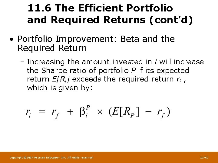
11. 6 The Efficient Portfolio and Required Returns (cont'd) • Portfolio Improvement: Beta and the Required Return – Increasing the amount invested in i will increase the Sharpe ratio of portfolio P if its expected return E[Ri] exceeds the required return ri , which is given by: Copyright © 2014 Pearson Education, Inc. All rights reserved. 11 -63

11. 6 The Efficient Portfolio and Required Returns (cont'd) • Portfolio Improvement: Beta and the Required Return – Required Return of i • The expected return that is necessary to compensate for the risk investment i will contribute to the portfolio. Copyright © 2014 Pearson Education, Inc. All rights reserved. 11 -64

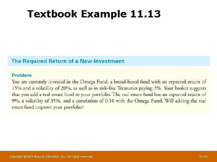
Textbook Example 11. 13 Copyright © 2014 Pearson Education, Inc. All rights reserved. 11 -65

Textbook Example 11. 13 (cont'd) Copyright © 2014 Pearson Education, Inc. All rights reserved. 11 -66

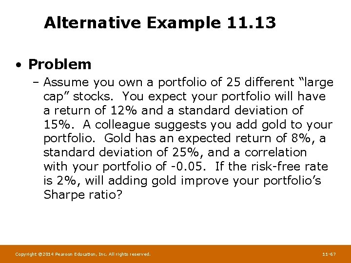
Alternative Example 11. 13 • Problem – Assume you own a portfolio of 25 different “large cap” stocks. You expect your portfolio will have a return of 12% and a standard deviation of 15%. A colleague suggests you add gold to your portfolio. Gold has an expected return of 8%, a standard deviation of 25%, and a correlation with your portfolio of -0. 05. If the risk-free rate is 2%, will adding gold improve your portfolio’s Sharpe ratio? Copyright © 2014 Pearson Education, Inc. All rights reserved. 11 -67

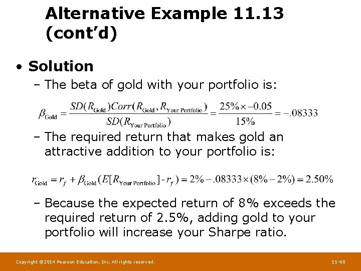
Alternative Example 11. 13 (cont’d) • Solution – The beta of gold with your portfolio is: – The required return that makes gold an attractive addition to your portfolio is: – Because the expected return of 8% exceeds the required return of 2. 5%, adding gold to your portfolio will increase your Sharpe ratio. Copyright © 2014 Pearson Education, Inc. All rights reserved. 11 -68

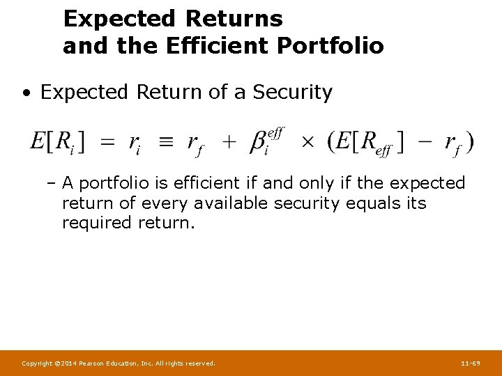
Expected Returns and the Efficient Portfolio • Expected Return of a Security – A portfolio is efficient if and only if the expected return of every available security equals its required return. Copyright © 2014 Pearson Education, Inc. All rights reserved. 11 -69

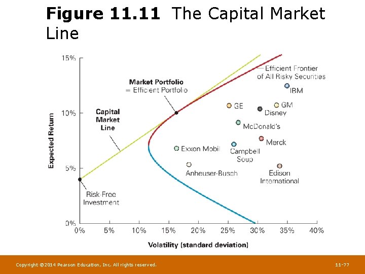
11. 7 The Capital Asset Pricing Model • The Capital Asset Pricing Model (CAPM) allows us to identify the efficient portfolio of risky assets without having any knowledge of the expected return of each security. • Instead, the CAPM uses the optimal choices investors make to identify the efficient portfolio as the market portfolio, the portfolio of all stocks and securities in the market. Copyright © 2014 Pearson Education, Inc. All rights reserved. 11 -70

The CAPM Assumptions • Three Main Assumptions – Assumption 1 • Investors can buy and sell all securities at competitive market prices (without incurring taxes or transactions costs) and can borrow and lend at the risk-free interest rate. Copyright © 2014 Pearson Education, Inc. All rights reserved. 11 -71

The CAPM Assumptions (cont'd) • Three Main Assumptions – Assumption 2 • Investors hold only efficient portfolios of traded securities—portfolios that yield the maximum expected return for a given level of volatility. Copyright © 2014 Pearson Education, Inc. All rights reserved. 11 -72

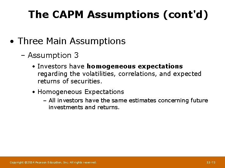
The CAPM Assumptions (cont'd) • Three Main Assumptions – Assumption 3 • Investors have homogeneous expectations regarding the volatilities, correlations, and expected returns of securities. • Homogeneous Expectations – All investors have the same estimates concerning future investments and returns. Copyright © 2014 Pearson Education, Inc. All rights reserved. 11 -73

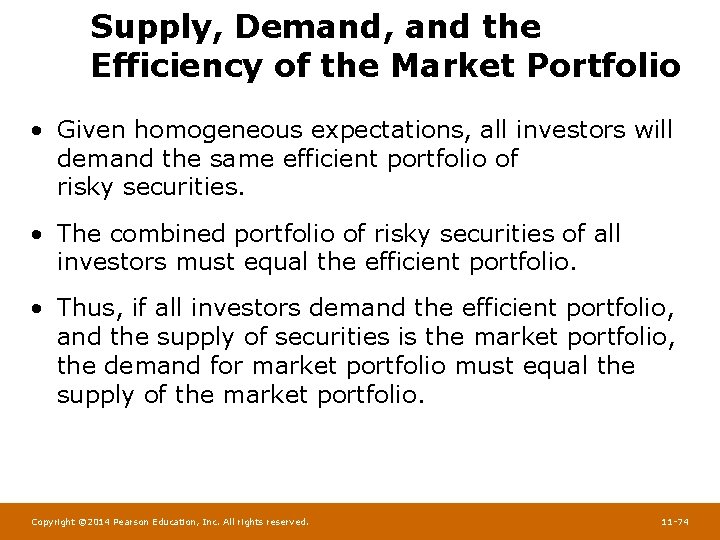
Supply, Demand, and the Efficiency of the Market Portfolio • Given homogeneous expectations, all investors will demand the same efficient portfolio of risky securities. • The combined portfolio of risky securities of all investors must equal the efficient portfolio. • Thus, if all investors demand the efficient portfolio, and the supply of securities is the market portfolio, the demand for market portfolio must equal the supply of the market portfolio. Copyright © 2014 Pearson Education, Inc. All rights reserved. 11 -74

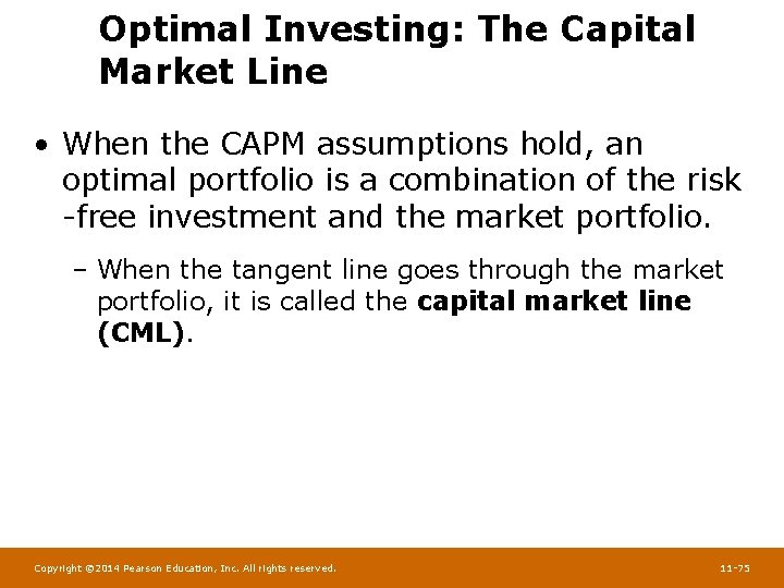
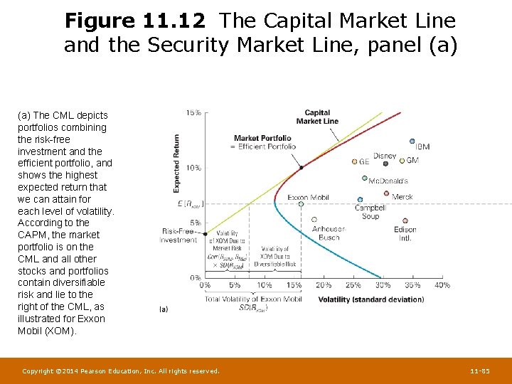
Optimal Investing: The Capital Market Line • When the CAPM assumptions hold, an optimal portfolio is a combination of the risk -free investment and the market portfolio. – When the tangent line goes through the market portfolio, it is called the capital market line (CML). Copyright © 2014 Pearson Education, Inc. All rights reserved. 11 -75

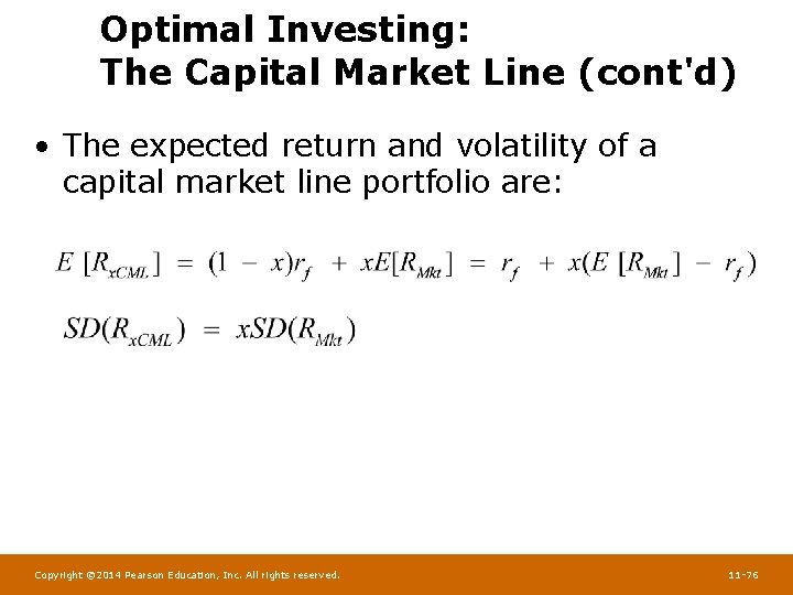
Optimal Investing: The Capital Market Line (cont'd) • The expected return and volatility of a capital market line portfolio are: Copyright © 2014 Pearson Education, Inc. All rights reserved. 11 -76

Figure 11. 11 The Capital Market Line Copyright © 2014 Pearson Education, Inc. All rights reserved. 11 -77

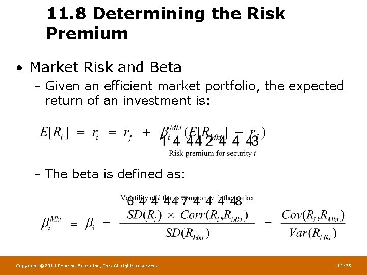
11. 8 Determining the Risk Premium • Market Risk and Beta – Given an efficient market portfolio, the expected return of an investment is: – The beta is defined as: Copyright © 2014 Pearson Education, Inc. All rights reserved. 11 -78

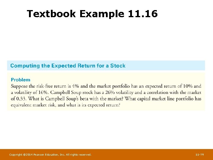
Textbook Example 11. 16 Copyright © 2014 Pearson Education, Inc. All rights reserved. 11 -79

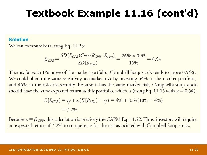
Textbook Example 11. 16 (cont'd) Copyright © 2014 Pearson Education, Inc. All rights reserved. 11 -80

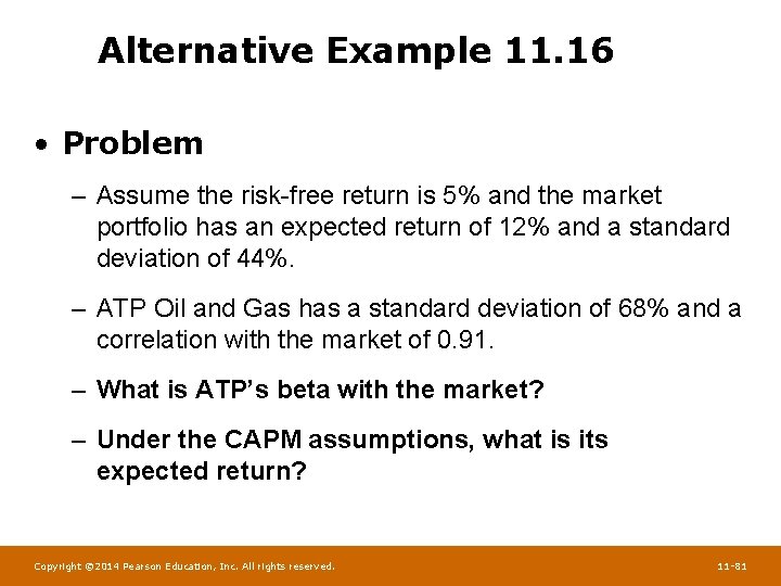
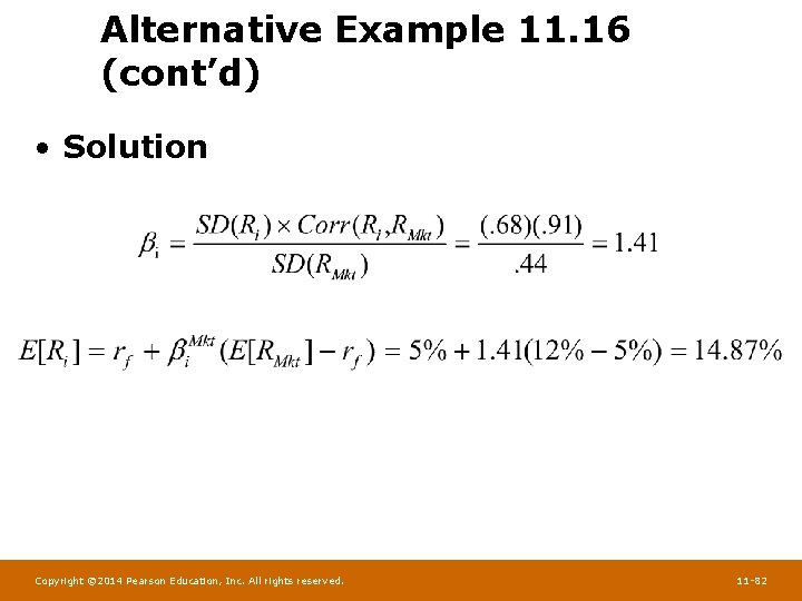
Alternative Example 11. 16 • Problem – Assume the risk-free return is 5% and the market portfolio has an expected return of 12% and a standard deviation of 44%. – ATP Oil and Gas has a standard deviation of 68% and a correlation with the market of 0. 91. – What is ATP’s beta with the market? – Under the CAPM assumptions, what is its expected return? Copyright © 2014 Pearson Education, Inc. All rights reserved. 11 -81

Alternative Example 11. 16 (cont’d) • Solution Copyright © 2014 Pearson Education, Inc. All rights reserved. 11 -82

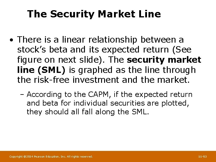
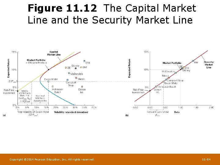
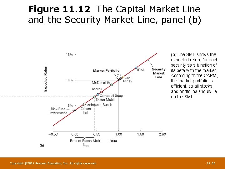
The Security Market Line • There is a linear relationship between a stock’s beta and its expected return (See figure on next slide). The security market line (SML) is graphed as the line through the risk-free investment and the market. – According to the CAPM, if the expected return and beta for individual securities are plotted, they should all fall along the SML. Copyright © 2014 Pearson Education, Inc. All rights reserved. 11 -83

Figure 11. 12 The Capital Market Line and the Security Market Line Copyright © 2014 Pearson Education, Inc. All rights reserved. 11 -84

Figure 11. 12 The Capital Market Line and the Security Market Line, panel (a) The CML depicts portfolios combining the risk-free investment and the efficient portfolio, and shows the highest expected return that we can attain for each level of volatility. According to the CAPM, the market portfolio is on the CML and all other stocks and portfolios contain diversifiable risk and lie to the right of the CML, as illustrated for Exxon Mobil (XOM). Copyright © 2014 Pearson Education, Inc. All rights reserved. 11 -85

Figure 11. 12 The Capital Market Line and the Security Market Line, panel (b) The SML shows the expected return for each security as a function of its beta with the market. According to the CAPM, the market portfolio is efficient, so all stocks and portfolios should lie on the SML. Copyright © 2014 Pearson Education, Inc. All rights reserved. 11 -86

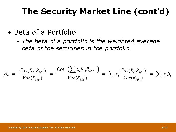
The Security Market Line (cont'd) • Beta of a Portfolio – The beta of a portfolio is the weighted average beta of the securities in the portfolio. Copyright © 2014 Pearson Education, Inc. All rights reserved. 11 -87

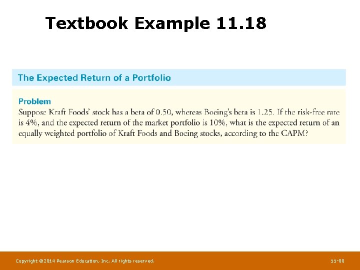
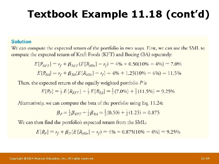
Textbook Example 11. 18 Copyright © 2014 Pearson Education, Inc. All rights reserved. 11 -88

Textbook Example 11. 18 (cont’d) Copyright © 2014 Pearson Education, Inc. All rights reserved. 11 -89

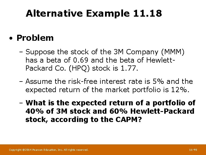
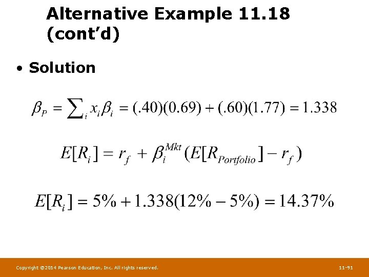
Alternative Example 11. 18 • Problem – Suppose the stock of the 3 M Company (MMM) has a beta of 0. 69 and the beta of Hewlett. Packard Co. (HPQ) stock is 1. 77. – Assume the risk-free interest rate is 5% and the expected return of the market portfolio is 12%. – What is the expected return of a portfolio of 40% of 3 M stock and 60% Hewlett-Packard stock, according to the CAPM? Copyright © 2014 Pearson Education, Inc. All rights reserved. 11 -90

Alternative Example 11. 18 (cont’d) • Solution Copyright © 2014 Pearson Education, Inc. All rights reserved. 11 -91

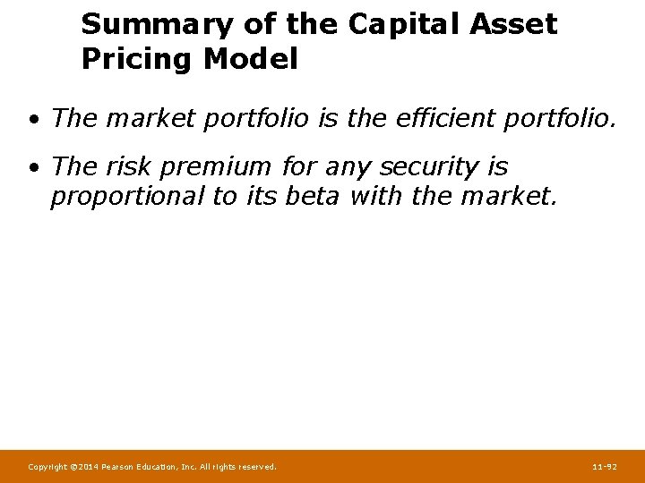
Summary of the Capital Asset Pricing Model • The market portfolio is the efficient portfolio. • The risk premium for any security is proportional to its beta with the market. Copyright © 2014 Pearson Education, Inc. All rights reserved. 11 -92