Chapter 11 n n Cash Flow Estimation Capital

Chapter 11 n n Cash Flow Estimation Capital Budgeting decisions must be based on cash flows not on accounting income Identify and use relevant cash flows, and ignore irrelevant ones. 1

Picking up Relevant Cash Flows Examples of Relevant Cash Flows n n n Opportunity costs The most valuable alternative that is given up if a particular investment is undertaken. These are relevant costs. Erosion (or Cannibalization) The cash flows of a new project that come at the expense of a firm’s existing projects. These are relevant costs. Shipping and Installation costs These are relevant costs. They also increase the depreciable basis of the purchased equipment. 2

An Example of Irrelevant Cash Flows Sunk cost A cost that has already been incurred and cannot be removed and therefore should not be considered in an investment decision 3

Incremental cash flows The difference between a firm’s future cash flows with a project or without the project. In general, they consist of: a. Operating Cash Flow b. Capital Spending c. Change in Net working capital 4

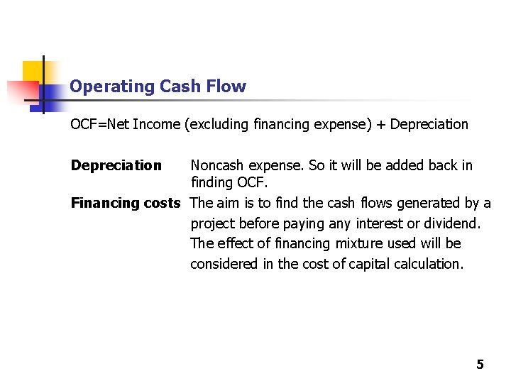
Operating Cash Flow OCF=Net Income (excluding financing expense) + Depreciation Noncash expense. So it will be added back in finding OCF. Financing costs The aim is to find the cash flows generated by a project before paying any interest or dividend. The effect of financing mixture used will be considered in the cost of capital calculation. 5

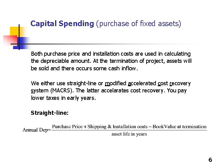
Capital Spending (purchase of fixed assets) Both purchase price and installation costs are used in calculating the depreciable amount. At the termination of project, assets will be sold and there occurs some cash inflow. We either use straight-line or modified accelerated cost recovery system (MACRS). The latter accelarates cost recovery. You pay lower taxes in early years. Straight-line: 6

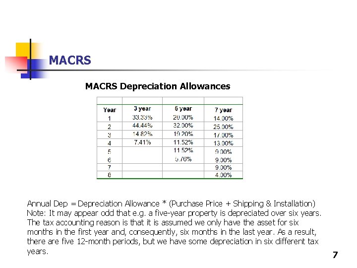
MACRS Depreciation Allowances Annual Dep = Depreciation Allowance * (Purchase Price + Shipping & Installation) Note: It may appear odd that e. g. a five-year property is depreciated over six years. The tax accounting reason is that it is assumed we only have the asset for six months in the first year and, consequently, six months in the last year. As a result, there are five 12 -month periods, but we have some depreciation in six different tax years. 7

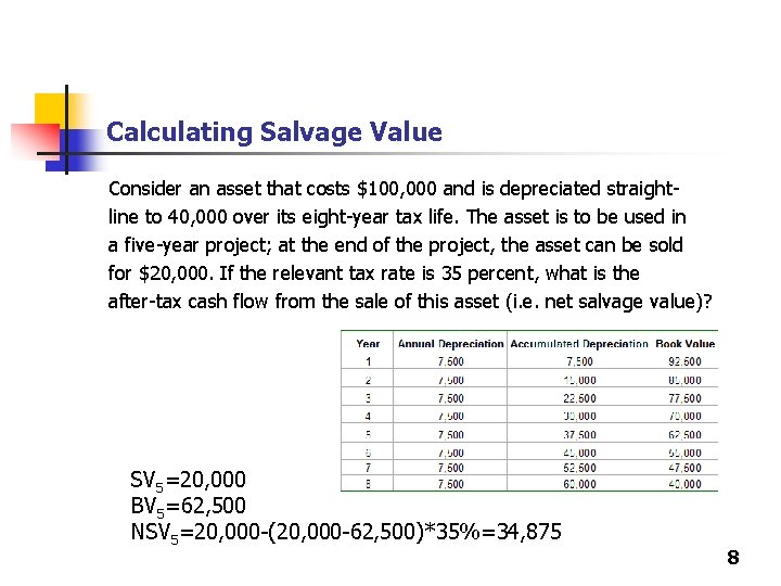
Calculating Salvage Value Consider an asset that costs $100, 000 and is depreciated straightline to 40, 000 over its eight-year tax life. The asset is to be used in a five-year project; at the end of the project, the asset can be sold for $20, 000. If the relevant tax rate is 35 percent, what is the after-tax cash flow from the sale of this asset (i. e. net salvage value)? SV 5=20, 000 BV 5=62, 500 NSV 5=20, 000 -(20, 000 -62, 500)*35%=34, 875 8

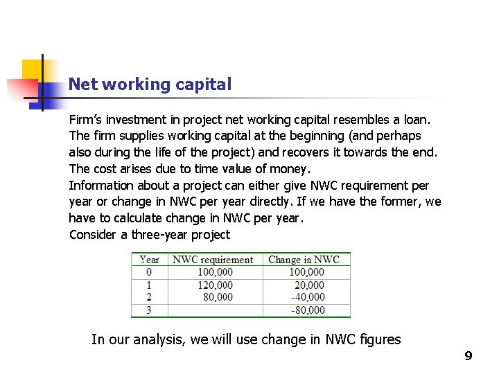
Net working capital Firm’s investment in project net working capital resembles a loan. The firm supplies working capital at the beginning (and perhaps also during the life of the project) and recovers it towards the end. The cost arises due to time value of money. Information about a project can either give NWC requirement per year or change in NWC per year directly. If we have the former, we have to calculate change in NWC per year. Consider a three-year project In our analysis, we will use change in NWC figures 9

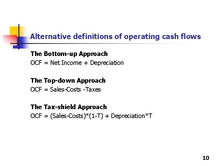
Alternative definitions of operating cash flows The Bottom-up Approach OCF = Net Income + Depreciation The Top-down Approach OCF = Sales-Costs -Taxes The Tax-shield Approach OCF = (Sales-Costs)*(1 -T) + Depreciation*T 10

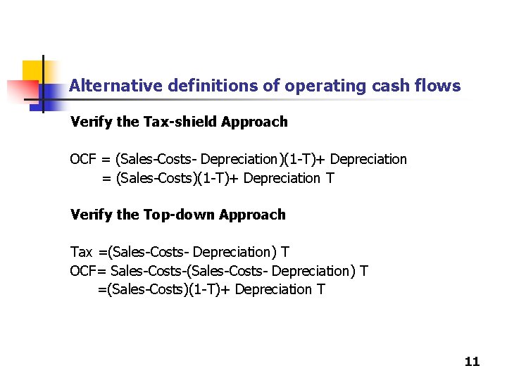
Alternative definitions of operating cash flows Verify the Tax-shield Approach OCF = (Sales-Costs- Depreciation)(1 -T)+ Depreciation = (Sales-Costs)(1 -T)+ Depreciation T Verify the Top-down Approach Tax =(Sales-Costs- Depreciation) T OCF= Sales-Costs-(Sales-Costs- Depreciation) T =(Sales-Costs)(1 -T)+ Depreciation T 11

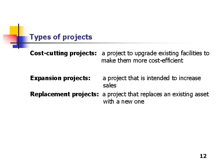
Types of projects Cost-cutting projects: a project to upgrade existing facilities to make them more cost-efficient Expansion projects: a project that is intended to increase sales Replacement projects: a project that replaces an existing asset with a new one 12

Examples Cost-Cutting Proposals Wally’s Water Works is looking at a new piping system with an installed cost of $180, 000. This cost will be depreciated straight-line to zero over the project’s five-year life, at the end of which the piping system can be scrapped for $25, 000. The piping system will save the firm $65, 000 per year in pretax operating costs, and the system requires an initial investment in net working capital of $17, 500. If the tax rate is 38 percent and the discount rate is 10 percent, what is the NPV of this project? See extra problems for examples on expansion and replacement projects 13

Risk Analysis We used our best guesses for parameter values to forecast NPV e. g. projected unit sales or projected savings in costs or projected salvage value etc. But realizations of parameter values will be different than our best guesses We can measure stand-alone risk It is the worst of 3 risk measures. But it is easiest to measure and all 3 measures are highly correlated. 14

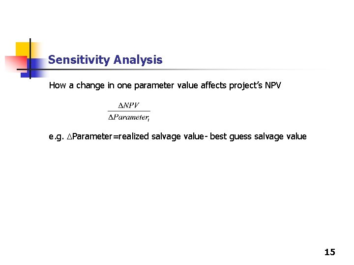
Sensitivity Analysis How a change in one parameter value affects project’s NPV e. g. Parameter=realized salvage value- best guess salvage value 15

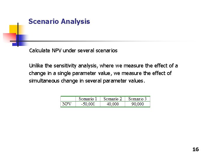
Scenario Analysis Calculate NPV under several scenarios Unlike the sensitivity analysis, where we measure the effect of a change in a single parameter value, we measure the effect of simultaneous change in several parameter values. 16

Monte Carlo Simulation Rather than using a single value for each parameter, you can specify a distribution for each parameter. Randomly sampled values are used to compute NPV over and over again. At the end, you get a distribution for NPV. This is analogous to scenario analysis, where we have possible scenarios. We sample a finite number of these scenarios. 17