Chapter 11 Inference for Distributions The onesample t

Chapter 11 Inference for Distributions

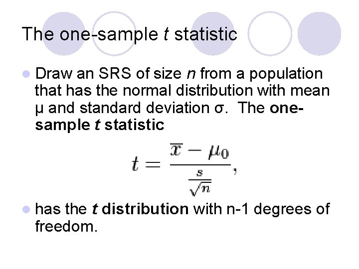
The one-sample t statistic l Draw an SRS of size n from a population that has the normal distribution with mean µ and standard deviation σ. The onesample t statistic l has the t distribution with n-1 degrees of freedom.

Key features of t distributions l Density curves are similar in shape to the standard normal curve l Spread is a bit greater than that of the standard normal distribution. l As the degrees of freedom increase, the density curve approaches the N(o, 1) curve more closely.

Using the t-table l What critical value from Table C would you use for a t-distribution with 18 degrees of freedom having probability 0. 90 to the left of t? l When using a t-table the probability given is to the right – we need 1 -0. 90 = 0. 10 with df of 18. t* = 1. 330

More on Using t-table l Suppose that we want to construct a 95% confidence interval for the mean µ of a population based on an SRS of size n=12. What critical value t should you use? t* = 2. 201

Constructing a confidence interval l Identify the population of interest and the parameter you want to draw conclusions about. l Choose the appropriate inference procedure. Verify the conditions for using the selected procedure l Carry out the inference procedure. l Interpret your results in the context of the problem.

Example 11. 2 l Auto Pollution: the major pollutants in auto exhaust are hydrocarbons, monoxide, and nitrogen oxide (NOX). l Given the NOX levels for a sample of lightduty engines of the same type, construct a 95% confidence interval for the mean amount of NOX emitted.

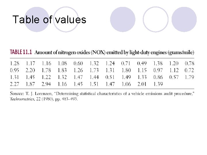
Table of values

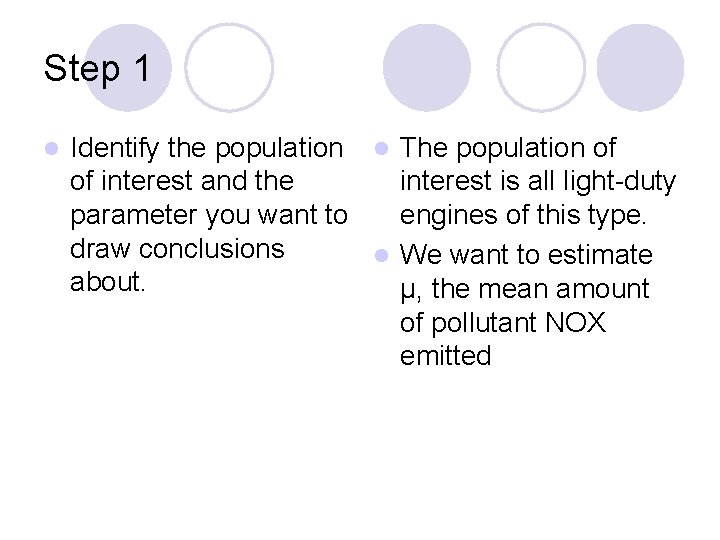
Step 1 l Identify the population l The population of of interest and the interest is all light-duty parameter you want to engines of this type. draw conclusions l We want to estimate about. µ, the mean amount of pollutant NOX emitted

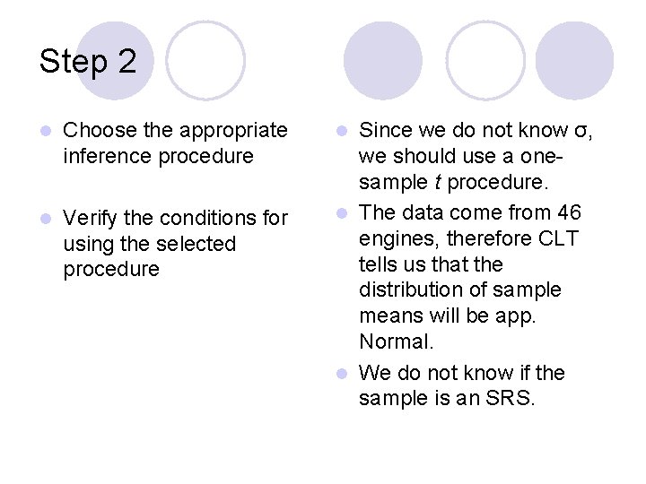
Step 2 l Choose the appropriate inference procedure l Verify the conditions for using the selected procedure Since we do not know σ, we should use a onesample t procedure. l The data come from 46 engines, therefore CLT tells us that the distribution of sample means will be app. Normal. l We do not know if the sample is an SRS. l

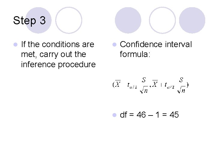
Step 3 l If the conditions are met, carry out the inference procedure l Confidence interval formula: l df = 46 – 1 = 45

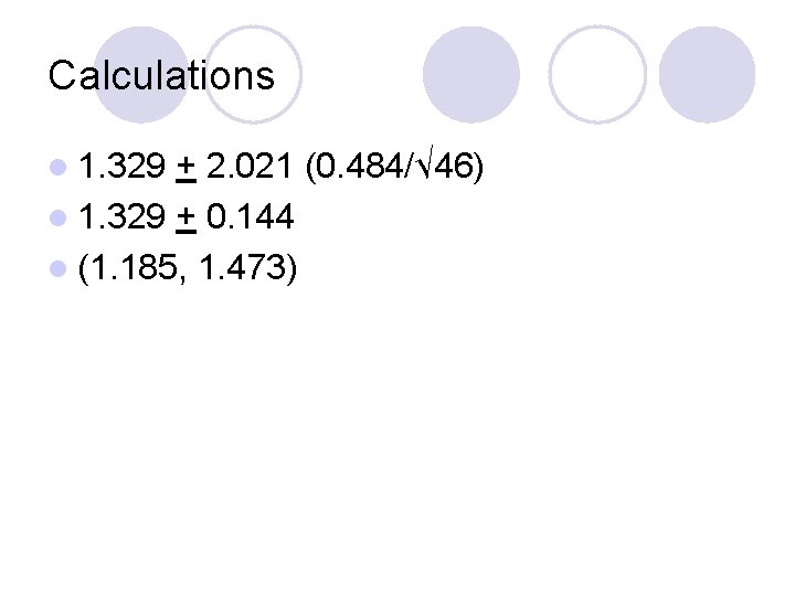
Calculations l 1. 329 + 2. 021 (0. 484/√ 46) l 1. 329 + 0. 144 l (1. 185, 1. 473)

Step 4 l Interpret your results in the context of the problem l We are 95% confident that the true mean level of nitrogen oxides emitted by this type of light-duty engine is between 1. 185 grams/mile and 1. 473 grams/mile.

Using Technology l Look at test under STAT and run a Tinterval for the previous problem.

Significance test for µ when σ is unknown l Cola makers test new recipes for loss of sweetness during storage. Following are the sweetness losses found by 10 tasters for one new cola recipe: l 2. 0 0. 4 0. 7 2. 0 -0. 4 l 2. 2 -1. 3 1. 2 1. 1 2. 3 l Are these good evidence that the cola lost sweetness?

Step 1 Identify the population l Tasters vary in their of interest and the perception of parameter you want to sweetness loss draw conclusions about. l State the null and l H 0: µDIFF = 0 alternative hypothesis in words and symbols l Ha: µDIFF > 0 l

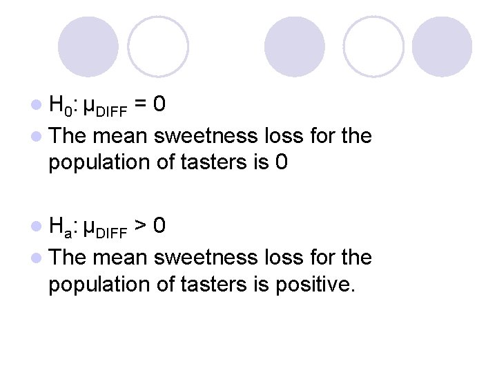
l H 0: µDIFF =0 l The mean sweetness loss for the population of tasters is 0 l Ha: µDIFF >0 l The mean sweetness loss for the population of tasters is positive.

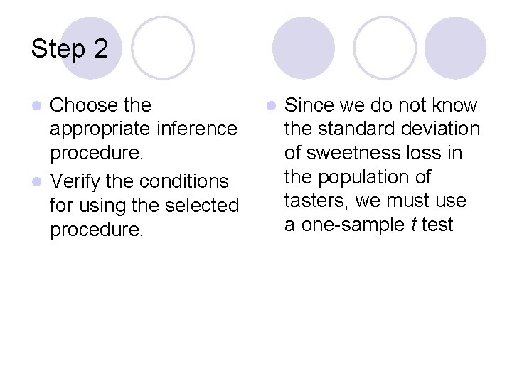
Step 2 Choose the appropriate inference procedure. l Verify the conditions for using the selected procedure. l l Since we do not know the standard deviation of sweetness loss in the population of tasters, we must use a one-sample t test

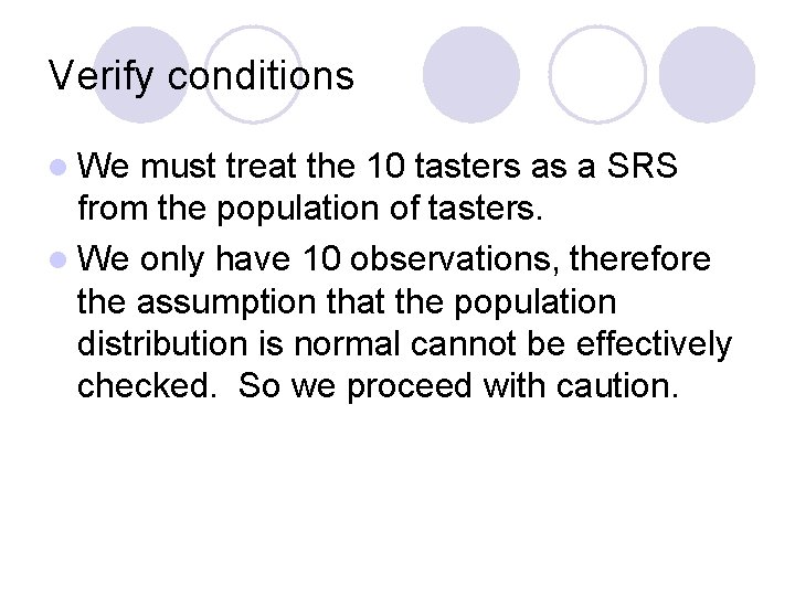
Verify conditions l We must treat the 10 tasters as a SRS from the population of tasters. l We only have 10 observations, therefore the assumption that the population distribution is normal cannot be effectively checked. So we proceed with caution.

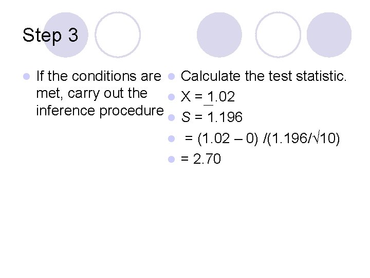
Step 3 l If the conditions are l Calculate the test statistic. met, carry out the l X = 1. 02 inference procedure l S = 1. 196 l = (1. 02 – 0) /(1. 196/√ 10) l = 2. 70

Step 3 continued l Find the P-value l The P-value for t=2. 70 and df = 10 -1 = 9 l It is somewhere between 0. 01 and 0. 02.

Step 4 l Interpret your results in the context of the problem l A P-value this low gives quite strong evident against the null hypothesis. We reject H 0 and conclude that the cola has lost sweetness during storage.

Exercises l 11. 7 and 11. 9

Matched pairs t procedure l In matched pairs design, subjects are matched in pairs and each treatment is given to one subject in each pair.

Robustness of t procedures l. A confidence interval or significance test is called robust if the confidence level or Pvalue does not change very much when the assumptions of the procedure are violated l Since mean and sample standard deviation are strongly influenced by outliers – the t-test will be also.

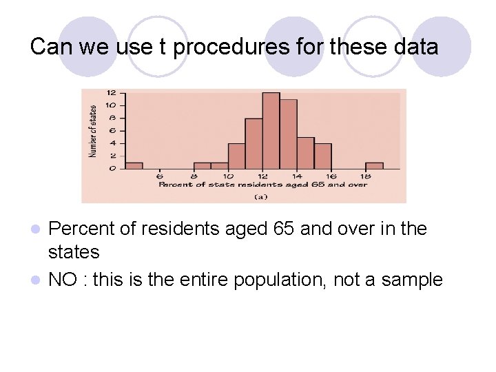
Can we use t procedures for these data Percent of residents aged 65 and over in the states l NO : this is the entire population, not a sample l

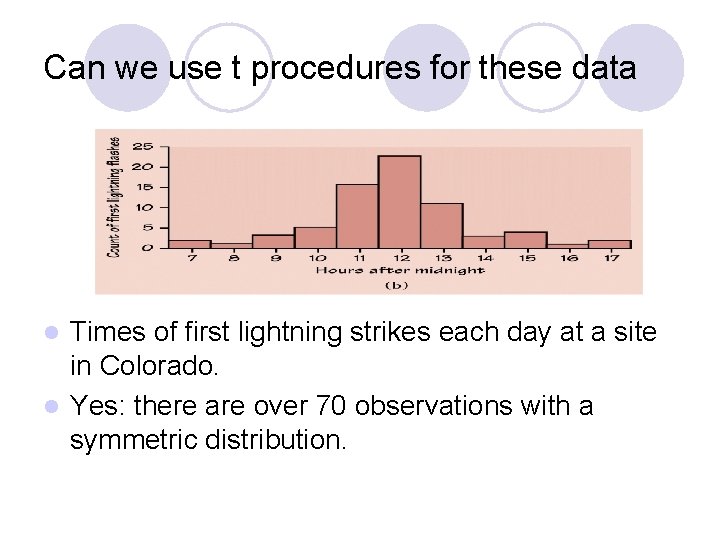
Can we use t procedures for these data Times of first lightning strikes each day at a site in Colorado. l Yes: there are over 70 observations with a symmetric distribution. l

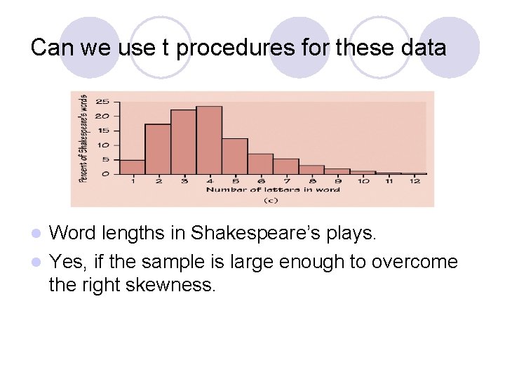
Can we use t procedures for these data Word lengths in Shakespeare’s plays. l Yes, if the sample is large enough to overcome the right skewness. l

Exercises to practice l 11. 17 and 11. 20