Chapter 11 Imperfect Competition 2004 Thomson LearningSouthWestern Imperfect

Chapter 11 Imperfect Competition © 2004 Thomson Learning/South-Western

Imperfect Competition l l Pricing in these markets falls between perfect competition and monopoly. Three topics considered: – – – 2 Pricing of homogeneous goods in markets with few firms. Product differentiation in these markets. How entry and exit affect long-run outcomes in imperfectly competitive markets.

Pricing of Homogeneous Goods l In this market a relatively few firms produce a single homogeneous good. – – l l 3 Assume demanders are price takers. Assume there are no transactions or informational costs. These assumptions result in a single equilibrium price for the good. Initially, assume a fixed, small number of identical firms.

Quasi-Competitive Model l 4 A model of oligopoly pricing in which each firm acts as a price taker even though there may be few firms is a quasi-competitive model. As a price taker, a firm will produce where price equals long-run marginal costs. This equilibrium will resemble the perfectly competitive solution, even with few firms.

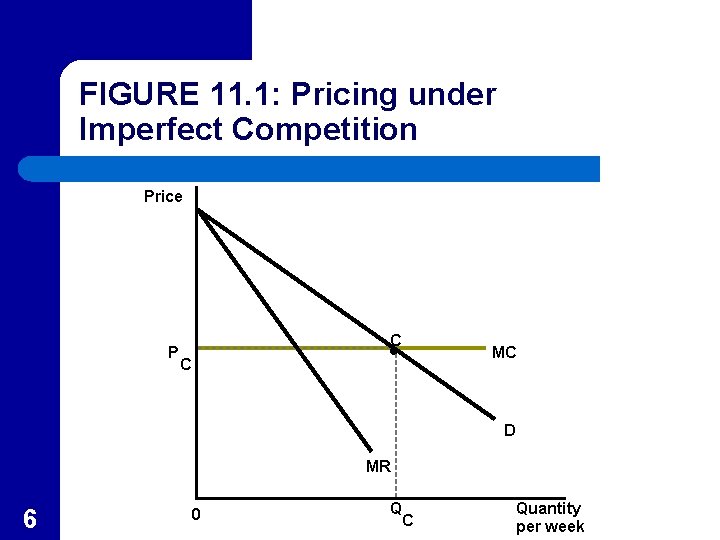
Quasi-Competitive Model l l In Figure 11. 1, the quasi-competitive equilibrium is PC (= MC), QC. This equilibrium represents the highest quantity and lowest price that can prevail in the long run given the demand curve D. – 5 A lower price would not be sustainable in the long run because it would not cover average costs.

FIGURE 11. 1: Pricing under Imperfect Competition Price P C C MC D MR 6 0 Q C Quantity per week

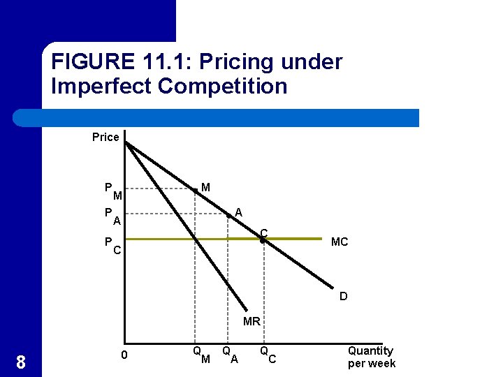
Cartel Model l l A model of pricing in which firms coordinate their decisions to act as a multiplant monopoly is the cartel model. Assuming marginal costs are constant and equal across firms, the cartel output is point M (the monopoly output) in Figure 11. 1. – 7 The plan would require a certain output by each firm and how to share the monopoly profits.

FIGURE 11. 1: Pricing under Imperfect Competition Price P P P M M A A C C MC D MR 8 0 Q M Q A Q C Quantity per week

Cartel Model l Maintaining this cartel solution poses three problems: – – Cartel formations may be illegal, as it is in the U. S. by Section I of the Sherman Act of 1890. It requires a considerable amount of costly information be available to the cartel. l l 9 The market demand function. Each firm’s marginal cost function.

Cartel Model – 10 The cartel solution may be fundamentally unstable. l Each member produces an output level for which price exceeds marginal cost. l Each member could increase its own profits by producing more output than allocated by the cartel. l If the cartel directors are not able to enforce their policies, the cartel my collapse.

APPLICATION 11. 1: The De Beers Cartel l l 11 In the 1870 s the discovery of the rich diamond fields in South Africa lead to major gem and industrial markets. After a competitive start, the ownership of the richest mines became incorporated into the De Beers Consolidated Mines which continues to dominate the world diamond trade.

APPLICATION 11. 1: The De Beers Cartel l Operation of the De Beers Cartel – – 12 Since the 1880 s diamonds found outside of South Africa are usually sold to De Beers who markets the diamonds to the final consumers through its central selling organization (CSO) in London. By controlling supply, the CSO maintains high prices which have been estimated to be as much as one thousand times marginal cost.

APPLICATION 11. 1: The De Beers Cartel l Dealing with Threats to the Cartel – – This large markup promotes threat of entry with any new diamond discovery. De Beers has used its market power to control would-be-chiselers. l l 13 They drove down prices when the former Soviet Union and Zaire tried market entry in the 1980 s. New finds in Australia were sold to the CSO rather than try to fight the cartel.

APPLICATION 11. 1: The De Beers Cartel l The Glamour of D Beers – – – 14 De Beers controls most print and television advertising, including “Diamonds Are Forever”. They convinced Japanese couples to adopt the western habit of buying engagement rings. De Beers has attempted to generate a brand name with customers to get consumers to judge De Beers diamonds superior to other suppliers.

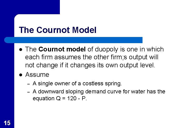
The Cournot Model l l The Cournot model of duopoly is one in which each firm assumes the other firm; s output will not change if it changes its own output level. Assume – – 15 A single owner of a costless spring. A downward sloping demand curve for water has the equation Q = 120 - P.

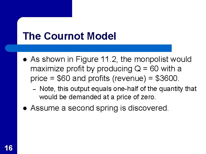
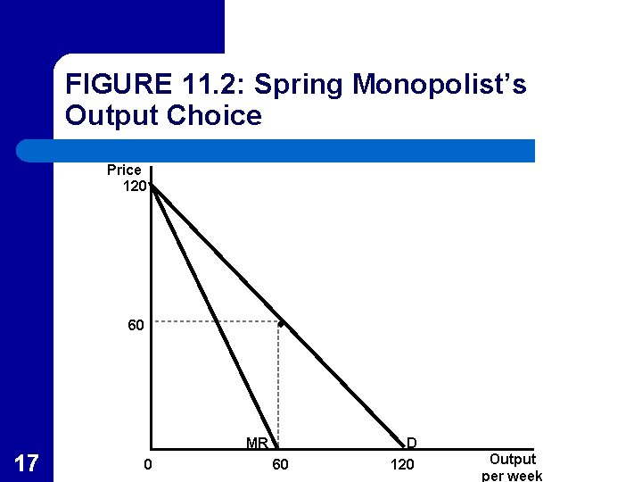
The Cournot Model l As shown in Figure 11. 2, the monpolist would maximize profit by producing Q = 60 with a price = $60 and profits (revenue) = $3600. – l 16 Note, this output equals one-half of the quantity that would be demanded at a price of zero. Assume a second spring is discovered.

FIGURE 11. 2: Spring Monopolist’s Output Choice Price 120 60 MR 17 0 60 D 120 Output per week

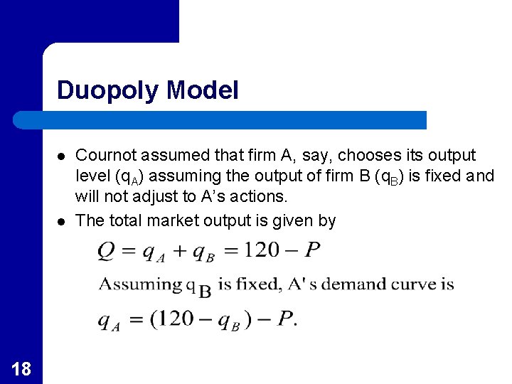
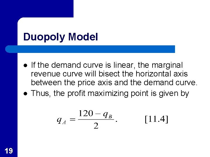
Duopoly Model l l 18 Cournot assumed that firm A, say, chooses its output level (q. A) assuming the output of firm B (q. B) is fixed and will not adjust to A’s actions. The total market output is given by

Duopoly Model l l 19 If the demand curve is linear, the marginal revenue curve will bisect the horizontal axis between the price axis and the demand curve. Thus, the profit maximizing point is given by

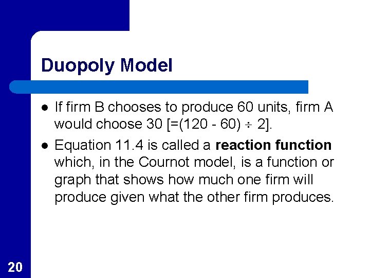
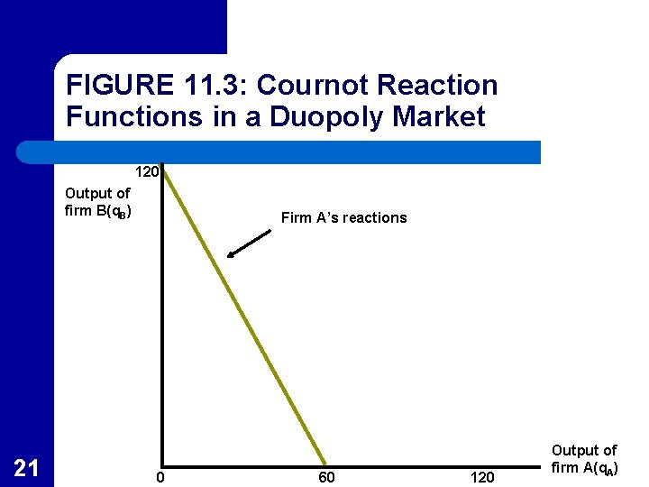
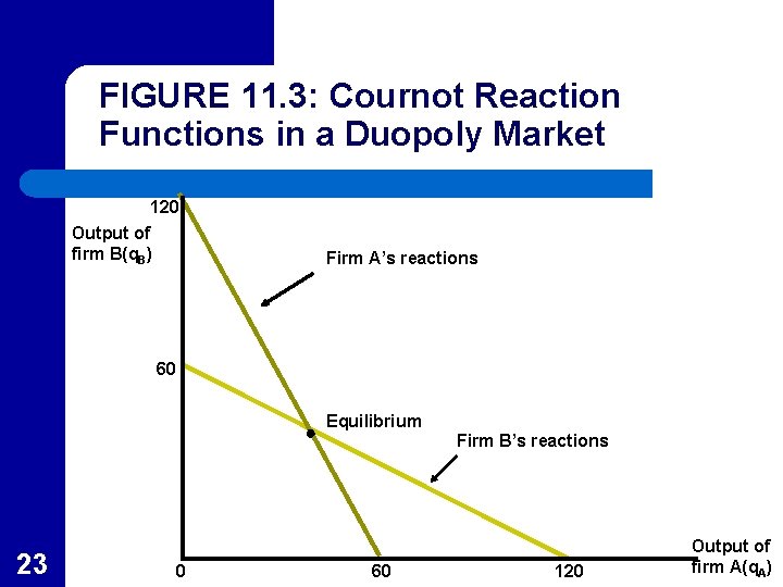
Duopoly Model l l 20 If firm B chooses to produce 60 units, firm A would choose 30 [=(120 - 60) 2]. Equation 11. 4 is called a reaction function which, in the Cournot model, is a function or graph that shows how much one firm will produce given what the other firm produces.

FIGURE 11. 3: Cournot Reaction Functions in a Duopoly Market 120 Output of firm B(q. B) 21 Firm A’s reactions 0 60 120 Output of firm A(q. A)

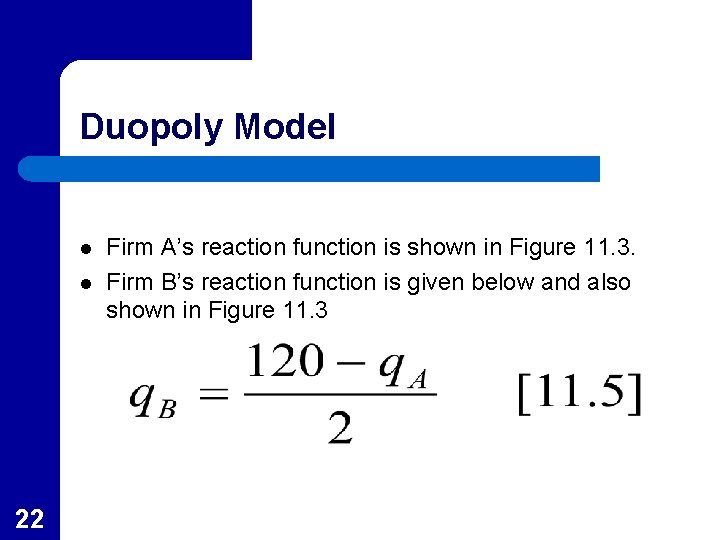
Duopoly Model l l 22 Firm A’s reaction function is shown in Figure 11. 3. Firm B’s reaction function is given below and also shown in Figure 11. 3

FIGURE 11. 3: Cournot Reaction Functions in a Duopoly Market 120 Output of firm B(q. B) Firm A’s reactions 60 Equilibrium Firm B’s reactions 23 0 60 120 Output of firm A(q. A)

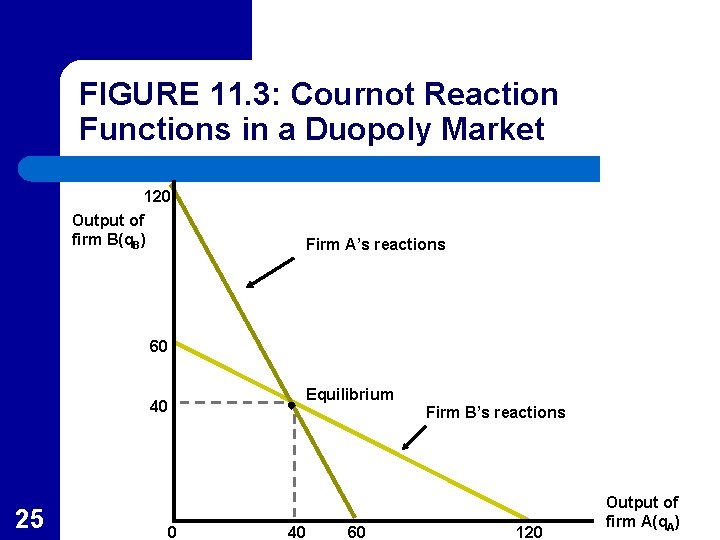
Cournot Equilibrium l l 24 The actions of the two firms are consistent with each other only at the point where the two lines intersect. The point of intersection is the Cournot equilibrium, a solution to the Cournot model in which each firm makes the correct assumption about what the other firm will produce.

FIGURE 11. 3: Cournot Reaction Functions in a Duopoly Market 120 Output of firm B(q. B) Firm A’s reactions 60 Equilibrium 40 25 Firm B’s reactions 0 40 60 120 Output of firm A(q. A)

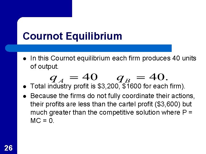
Cournot Equilibrium l In this Cournot equilibrium each firm produces 40 units of output. l Total industry profit is $3, 200, $1600 for each firm). Because the firms do not fully coordinate their actions, their profits are less than the cartel profit ($3, 600) but much greater than the competitive solution where P = MC = 0. l 26

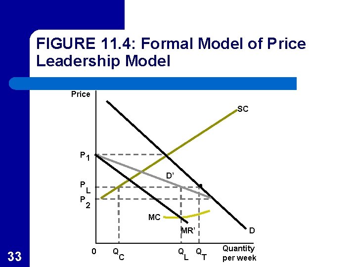
Price Leadership Model l l 27 A model in which one dominant firm takes reactions of all other firms into account in its output and pricing decisions is the price leadership model. A formal model assumes the industry is composed of a single price-setting leader and a competitive fringe which is a group of firms that act as price takers.

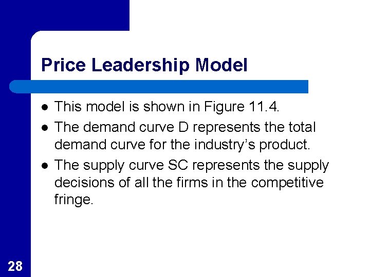
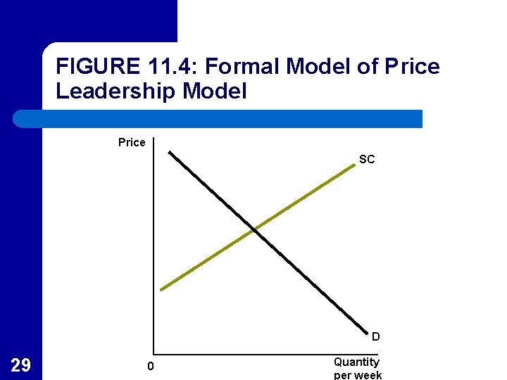
Price Leadership Model l 28 This model is shown in Figure 11. 4. The demand curve D represents the total demand curve for the industry’s product. The supply curve SC represents the supply decisions of all the firms in the competitive fringe.

FIGURE 11. 4: Formal Model of Price Leadership Model Price SC D 29 0 Quantity per week

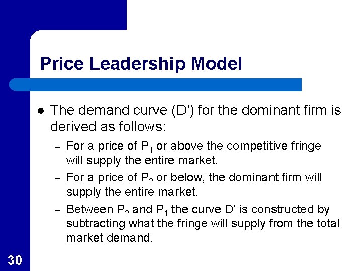
Price Leadership Model l The demand curve (D’) for the dominant firm is derived as follows: – – – 30 For a price of P 1 or above the competitive fringe will supply the entire market. For a price of P 2 or below, the dominant firm will supply the entire market. Between P 2 and P 1 the curve D’ is constructed by subtracting what the fringe will supply from the total market demand.

FIGURE 11. 4: Formal Model of Price Leadership Model Price SC P 1 D’ P 2 D 31 0 Quantity per week

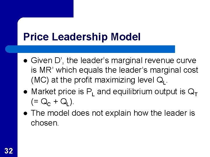
Price Leadership Model l 32 Given D’, the leader’s marginal revenue curve is MR’ which equals the leader’s marginal cost (MC) at the profit maximizing level QL. Market price is PL and equilibrium output is QT (= QC + QL). The model does not explain how the leader is chosen.

FIGURE 11. 4: Formal Model of Price Leadership Model Price SC P 1 D’ P P L 2 MC MR’ 33 0 Q C Q Q L T D Quantity per week

APPLICATION 11. 2: Cournot in California l Borenstein and Bushnell paper: Perhaps the most elaborate attempt at modeling the impact of electricity deregulation in California. – – 34 Authors focus on competition between the three major electricity-generating firms. They argue that the smaller suppliers can be treated as competitive suppliers but that the major in-state producers behave in the way assumed in the Cournot model.

APPLICATION 11. 2: Cournot in California l l 35 Borenstein and Bushnell show that under certain circumstances there is substantial market power in California wholesale electricity markets. One way to measure that power is by the Lerner Index, the ratio (P – MC/P). The authors showed with the Lerner Index that during peak periods, equilibrium in these markets is far from the competitive ideal. They also show that market power can be significantly restrained by larger price elasticities of demand for electricity.

Product Differentiation: Market Definition and Firms Choices l l l 36 A product group is a set of differentiated products that are highly substitutable for one another. Assume few firms in each product group. Firms will incur additional costs to differentiate their product up to the point where the additional revenue from this activity equals the marginal cost.

Product Differentiation: Market Equilibrium l l The demand curve for each firm depends on the prices and product differentiation activities of its competitors. The firm’s demand curve may shift frequently, and its position at any point in time may only be partially understood. – 37 Each firm must make assumptions about its competitors’ actions, and whatever one firm decides may affect its competitor’s actions.

APPLICATION 11. 3: Price Leadership in Financial Markets l The Prime Rate at New York Commercial Banks – – 38 Major New York commercial banks quote a “prime rate” which purports to be the interest rate that they charge on loans to their most creditworthy customers. Recent research indicates actual pricing is more complex, but the prime provides a visible and influential indicator or rate change.

APPLICATION 11. 3: Price Leadership in Financial Markets l l 39 While rates changes are sluggish, when “large” changes (0. 25 or more) are required one of the major banks will act like a leader and announce a new prime rate on a trial basis. After a few days, either most banks will follow or the initiator will return to its old rate.

APPLICATION 11. 3: Price Leadership in Financial Markets – – – 40 A number of researchers have found that rates tend to rise soon after an increase in bank costs, but decline only slowly when costs fall. Similarly, a rise in the prime tends to hurt the stock prices of banks that increase because the increase signals that profits hare being squeezed by costs. Alternatively, stock prices rise when the prime rate falls.

APPLICATION 11. 3: Price Leadership in Financial Markets l Price Leadership in the Foreign Exchange Market – – 41 The large market for world currencies is dominated by major financial institutions and is heavily influenced by the “intervention” of various nations’ central banks. Because central bank intervention is not announced in advance, well informed traders may have an information market advantage.

APPLICATION 11. 3: Price Leadership in Financial Markets – – In a study of the German Mark (DM), an author found that one bank tended to pay the role of leader in setting the DM/$ exchange rate. This leadership role arose because of the bank’s ability to foresee intervention by the German central bank in exchange markets. l 42 Quoted exchange rate between 25 and 60 minutes before the intervention were copied by other banks, while within 25 minutes (with information more diffused) no clear cut pattern emerged.

APPLICATION 11. 4: Competition in Breakfast Space l Industrial Concentration – – – 43 Three major firms control approximately 80 percent of the market. Returns on invested capital are more than double those of the average industry. It is unclear why the market is not more competitive since there do not seem to be any major economies of scale and no obvious barriers to entry.

APPLICATION 11. 4: Competition in Breakfast Space l The FTC Complaint and Product Differentiation – In 1972 the U. S. Federal Trade Commission (FTC) claimed the largest producers actions tended to establish monopoly-like conditions. l l 44 Proliferation of new, highly advertised, brands left no room for potential new entrants. Brand identification also prevented new entrants from duplicating existing cereal.

APPLICATION 11. 4: Competition in Breakfast Space l Demise of the Legal Case – – – l 45 Firms claimed that they were engaging in active competition by creating new cereal brands. Also, many new “natural” cereals did enter the market in the 1970 s. The case was quietly dropped in 1982. Recent studies still indicate a lack of competition and continued higher profits.

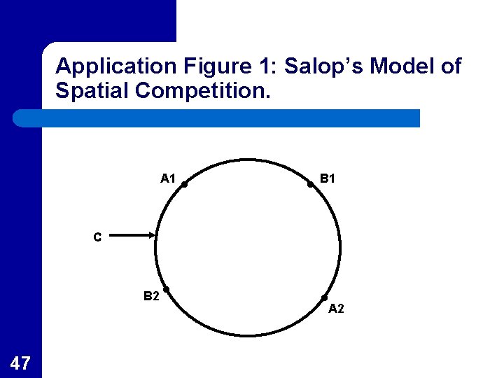
APPLICATION 11. 4: Competition in Breakfast Space l l l 46 One of illustrating the contention that major firms so proliferated their brands so as to keep potential competitors out was developed by S. Salop. Figure 1 depicts consumers evenly located along the circle which may represent an actual geographic space or product space. The presence of two firms (A and B) with two products each deters entry by C.

Application Figure 1: Salop’s Model of Spatial Competition. A 1 C . B 2 47 . . B 1 . A 2

Product Differentiation: Entry by New Firms l l l 48 The degree to which firms can enter the market plays an important role. Even with few firms, to the extent that entry is possible, long-run profits are constrained. If entry is completely costless, long-run economic profits will be zero (as in the competitive case).

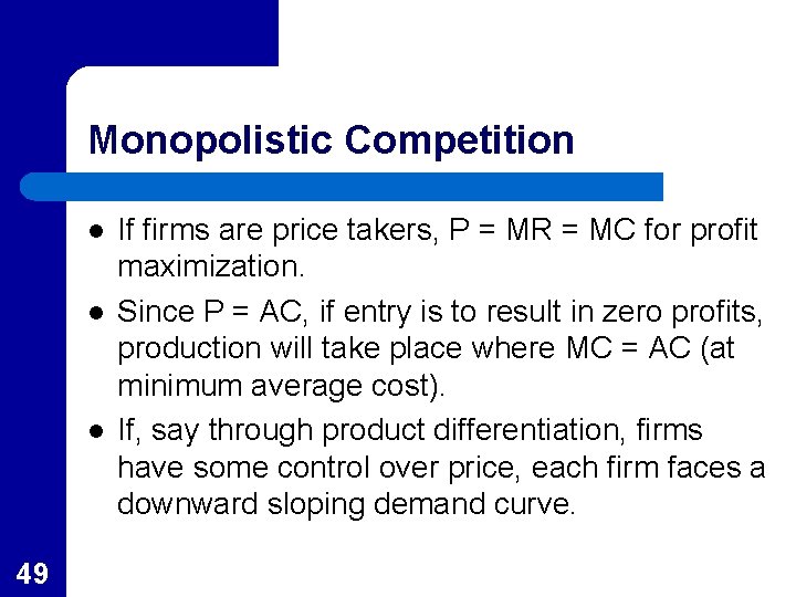
Monopolistic Competition l l l 49 If firms are price takers, P = MR = MC for profit maximization. Since P = AC, if entry is to result in zero profits, production will take place where MC = AC (at minimum average cost). If, say through product differentiation, firms have some control over price, each firm faces a downward sloping demand curve.

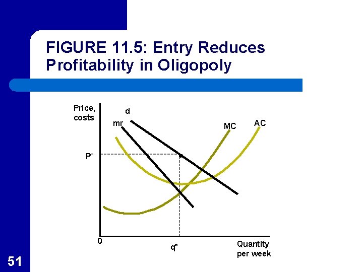
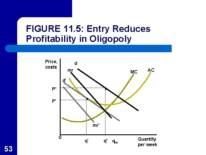
Monopolistic Competition l l l 50 Entry still may reduce profits to zero, but production at minimum cost is not assured. Monopolistic competition is a market in which each firm faces a negatively sloped demand curve and there are no barriers to entry. This type of market is illustrated in Figure 11. 5.

FIGURE 11. 5: Entry Reduces Profitability in Oligopoly Price, costs d mr MC AC P* 0 51 q* Quantity per week

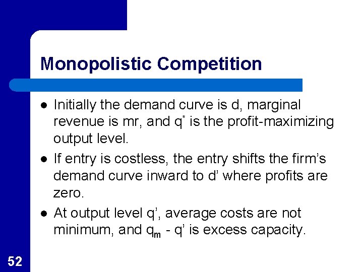
Monopolistic Competition l l l 52 Initially the demand curve is d, marginal revenue is mr, and q* is the profit-maximizing output level. If entry is costless, the entry shifts the firm’s demand curve inward to d’ where profits are zero. At output level q’, average costs are not minimum, and qm - q’ is excess capacity.

FIGURE 11. 5: Entry Reduces Profitability in Oligopoly Price, costs d mr MC AC d’ P* P’ mr’ 0 53 q’ q* qm Quantity per week

Sustainability of Monopolistic Competition l l 54 Monopolistic competition focuses only on the behavior of actual entrants but ignores the effects of potential entrants. A broader perspective of the “ invisible hand” is the distinction between competition in the market and competition for the market.

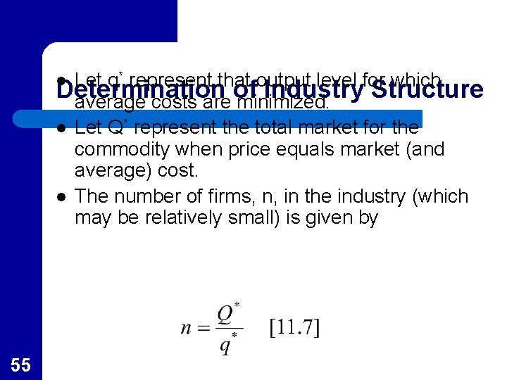
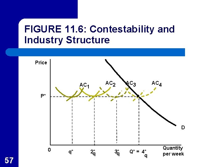
Let q* represent that output level for which Determination of Industry Structure average costs are minimized. l Let Q* represent the total market for the commodity when price equals market (and average) cost. l The number of firms, n, in the industry (which may be relatively small) is given by l 55

Determination of Industry Structure l l l 56 As shown in Figure 11. 6, for example, only four firms fulfill the market demand Q*. The contestability assumption will ensure competitive behavior even though firms may recognize strategic relationships among themselves. The potential for entrants constrains the types of behavior that are possible.

FIGURE 11. 6: Contestability and Industry Structure Price AC 2 AC 1 AC 3 AC 4 P* D 0 57 q* 2* q 3* q Q* = 4* q Quantity per week

APPLICATION 11. 4: Airline Deregulation Revisited l Airlines Contestability – – 58 Since planes are mobile, they can be moved into a market that promises excess profits. Such potential entry should hold prices at competitive levels even with few firms. However, terminal facilities are market specific and brand loyalty appears to exist. Also, some major airports have limited potential for growth.

APPLICATION 11. 4: Airline Deregulation Revisited l Effects of Deregulation – – 59 Studies suggest that fares declined after deregulation with one study suggesting yearly gains to customers of about $8. 6 billion. However, this study found that additional welfare gains of about $2. 5 billion were not realized because of the limitations of landing slots and computer reservations systems may aid in price collusion among major airlines.

APPLICATION 11. 4: Airline Deregulation Revisited l Trend in Airline Competition – – – 60 Many new airlines entered after the 1978 deregulation, but they were often consolidated into larger carriers. Several existing airlines went out of business. The hub-and-spoke designs of flight networks were introduced which has lead to dominance of one or two airlines in a hub city which may have resulted in higher fares.

Barriers to Entry l l The existence of barriers to entry change the type of analysis. In addition to those previously discussed, barriers include brand loyalty and strategic pricing. – 61 Firms may drive out potential entrants with low prices followed later by price increases or they may buy up smaller firms.