Chapter 11 Experimental Design and Analysis of Variance

Chapter 11 Experimental Design and Analysis of Variance Mc. Graw-Hill/Irwin Copyright © 2009 by The Mc. Graw-Hill Companies, Inc. All Rights Reserved.

Experimental Design and Analysis of Variance 11. 1 Basic Concepts of Experimental Design 11. 2 One-Way Analysis of Variance 11. 3 The Randomized Block Design 11. 4 Two-Way Analysis of Variance 11 -2

Basic Concepts of Experimental Design • Up until now, we have considered only two ways of collecting and comparing data: – Using independent random samples – Using paired (or matched) samples • Often data is collected as the result of an experiment – To systematically study how one or more factors (variables) influence the variable that is being studied 11 -3

Experimental Design #2 • In an experiment, there is strict control over the factors contributing to the experiment – The values or levels of the factors are called treatments • For example, in testing a medical drug, the experimenters decide which participants in the test get the drug and which ones get the placebo, instead of leaving the choice to the subjects • The object is to compare and estimate the effects of different treatments on the response variable 11 -4

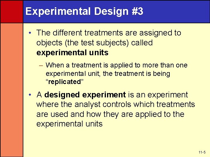
Experimental Design #3 • The different treatments are assigned to objects (the test subjects) called experimental units – When a treatment is applied to more than one experimental unit, the treatment is being “replicated” • A designed experiment is an experiment where the analyst controls which treatments are used and how they are applied to the experimental units 11 -5

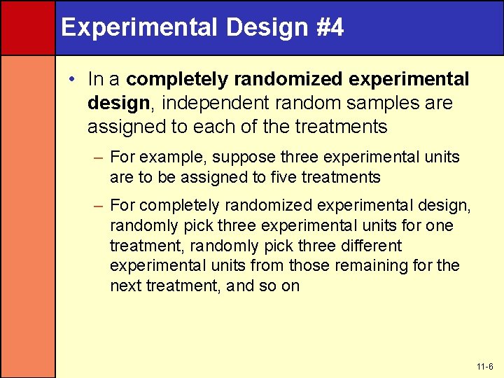
Experimental Design #4 • In a completely randomized experimental design, independent random samples are assigned to each of the treatments – For example, suppose three experimental units are to be assigned to five treatments – For completely randomized experimental design, randomly pick three experimental units for one treatment, randomly pick three different experimental units from those remaining for the next treatment, and so on 11 -6

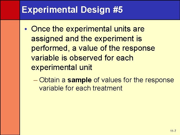
Experimental Design #5 • Once the experimental units are assigned and the experiment is performed, a value of the response variable is observed for each experimental unit – Obtain a sample of values for the response variable for each treatment 11 -7

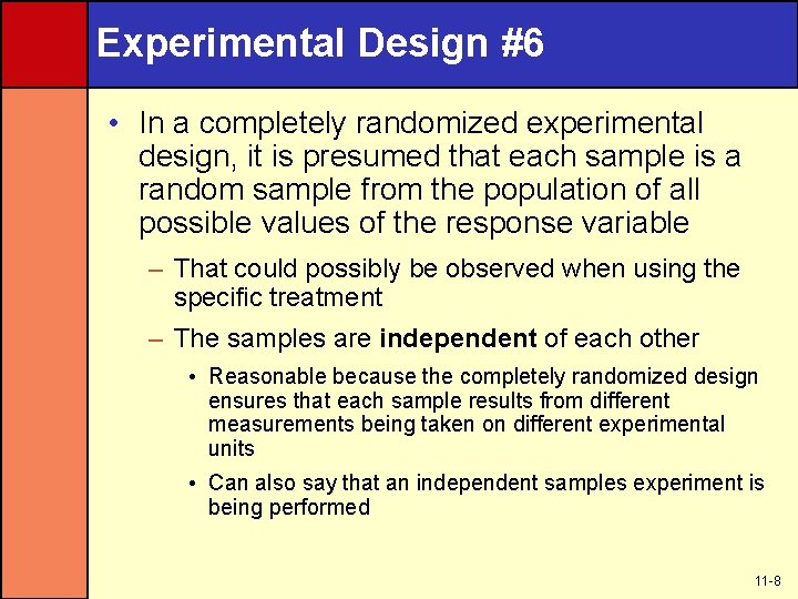
Experimental Design #6 • In a completely randomized experimental design, it is presumed that each sample is a random sample from the population of all possible values of the response variable – That could possibly be observed when using the specific treatment – The samples are independent of each other • Reasonable because the completely randomized design ensures that each sample results from different measurements being taken on different experimental units • Can also say that an independent samples experiment is being performed 11 -8

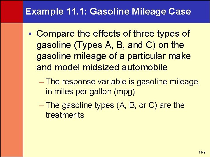
Example 11. 1: Gasoline Mileage Case • Compare the effects of three types of gasoline (Types A, B, and C) on the gasoline mileage of a particular make and model midsized automobile – The response variable is gasoline mileage, in miles per gallon (mpg) – The gasoline types (A, B, or C) are the treatments 11 -9

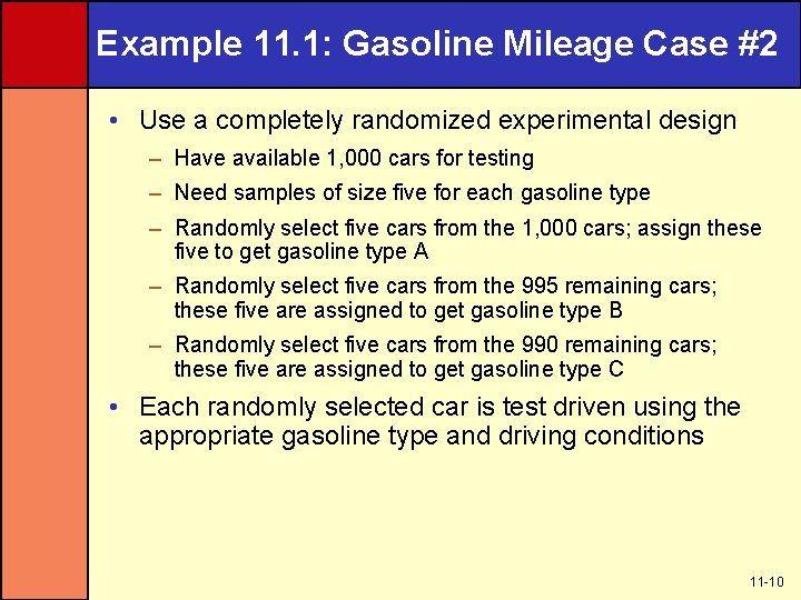
Example 11. 1: Gasoline Mileage Case #2 • Use a completely randomized experimental design – Have available 1, 000 cars for testing – Need samples of size five for each gasoline type – Randomly select five cars from the 1, 000 cars; assign these five to get gasoline type A – Randomly select five cars from the 995 remaining cars; these five are assigned to get gasoline type B – Randomly select five cars from the 990 remaining cars; these five are assigned to get gasoline type C • Each randomly selected car is test driven using the appropriate gasoline type and driving conditions 11 -10

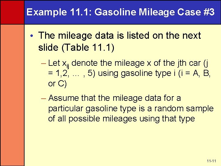
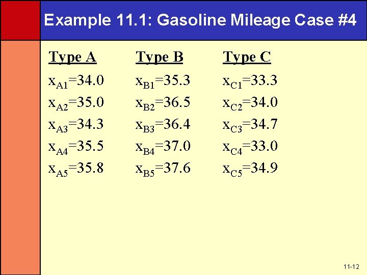
Example 11. 1: Gasoline Mileage Case #3 • The mileage data is listed on the next slide (Table 11. 1) – Let xij denote the mileage x of the jth car (j = 1, 2, … , 5) using gasoline type i (i = A, B, or C) – Assume that the mileage data for a particular gasoline type is a random sample of all possible mileages using that type 11 -11

Example 11. 1: Gasoline Mileage Case #4 Type A Type B Type C x. A 1=34. 0 x. A 2=35. 0 x. A 3=34. 3 x. A 4=35. 5 x. A 5=35. 8 x. B 1=35. 3 x. B 2=36. 5 x. B 3=36. 4 x. B 4=37. 0 x. B 5=37. 6 x. C 1=33. 3 x. C 2=34. 0 x. C 3=34. 7 x. C 4=33. 0 x. C 5=34. 9 11 -12

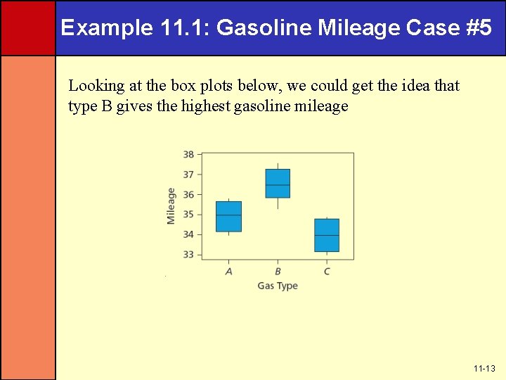
Example 11. 1: Gasoline Mileage Case #5 Looking at the box plots below, we could get the idea that type B gives the highest gasoline mileage 11 -13

One-Way Analysis of Variance • Want to study the effects of all p treatments on a response variable – For each treatment, find the mean and standard deviation of all possible values of the response variable when using that treatment – For treatment i, find treatment mean µi • One-way analysis of variance estimates and compares the effects of the different treatments on the response variable – By estimating and comparing the treatment means µ 1, µ 2, …, µp – One-way analysis of variance, or one-way ANOVA 11 -14

Example 11. 4: Gasoline Mileage Case • The mean of a sample is the point estimate for the corresponding treatment mean x. A = 34. 92 mpg estimates m. A x. B = 36. 56 mpg estimates m. B x. C = 33. 98 mpg estimates m. C 11 -15

Example 11. 4: Gasoline Mileage Case Continued • The standard deviation of a sample is the point estimate for the corresponding treatment standard estimates s. A = 0. 7662 mpg estimates σA s. B = 0. 8503 mpg estimates σB s. C = 0. 8349 mpg estimates σC 11 -16

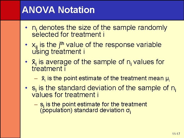
ANOVA Notation • ni denotes the size of the sample randomly selected for treatment i • xij is the jth value of the response variable using treatment i • xi is average of the sample of ni values for treatment i – xi is the point estimate of the treatment mean µi • si is the standard deviation of the sample of ni values for treatment i – si is the point estimate for the treatment (population) standard deviation σi 11 -17

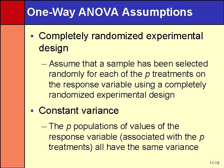
One-Way ANOVA Assumptions • Completely randomized experimental design – Assume that a sample has been selected randomly for each of the p treatments on the response variable using a completely randomized experimental design • Constant variance – The p populations of values of the response variable (associated with the p treatments) all have the same variance 11 -18

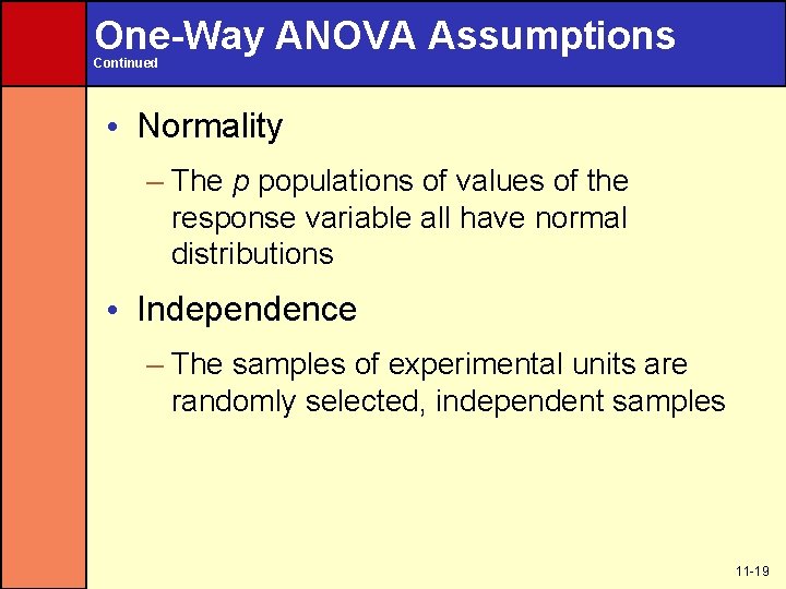
One-Way ANOVA Assumptions Continued • Normality – The p populations of values of the response variable all have normal distributions • Independence – The samples of experimental units are randomly selected, independent samples 11 -19

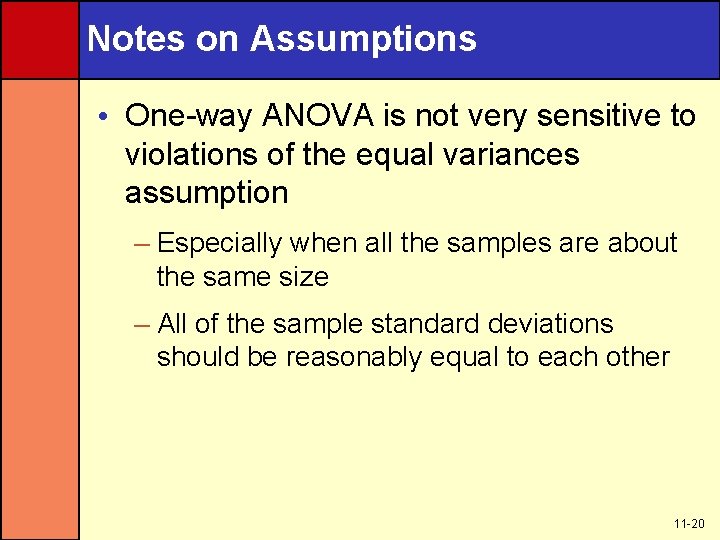
Notes on Assumptions • One-way ANOVA is not very sensitive to violations of the equal variances assumption – Especially when all the samples are about the same size – All of the sample standard deviations should be reasonably equal to each other 11 -20

Notes on Assumptions Continued • Normality is not crucial – ANOVA results are approximately valid for mound-shaped distributions • If the sample distributions are reasonably symmetric and if there are no outliers, then ANOVA results are valid for even small samples • For gasoline mileages, the assumptions are roughly satisfied 11 -21

Testing for Significant Differences Between Treatment Means • Are there any statistically significant differences between the sample (treatment) means? • The null hypothesis is that the mean of all p treatments are the same – H 0: µ 1 = µ 2 = … = µ p • The alternative is that some (or all, but at least two) of the p treatments have different effects on the mean response – Ha: at least two of µ 1, µ 2 , …, µp differ 11 -22

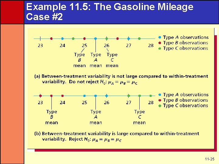
Testing for Significant Differences Between Treatment Means Continued • Compare the between-treatment variability to the within-treatment variability – Between-treatment variability is the variability of the sample means from sample to sample – Within-treatment variability is the variability of the treatments (that is, the values) within each sample 11 -23

Example 11. 5: The Gasoline Mileage Case • In Figure 11. 1(a), (next slide) the betweentreatment variability is not large compared to the within-treatment variability – The between-treatment variability could be the result of sampling variability – Do not have enough evidence to reject H 0: μ A = μ B = μ C • In figure 11. 1(b), between-treatment variability is large compared to the within-treatment variability – May have enough evidence to reject H 0 in favor of Ha: at least two of μA, μB, μC differ 11 -24

Example 11. 5: The Gasoline Mileage Case #2 11 -25

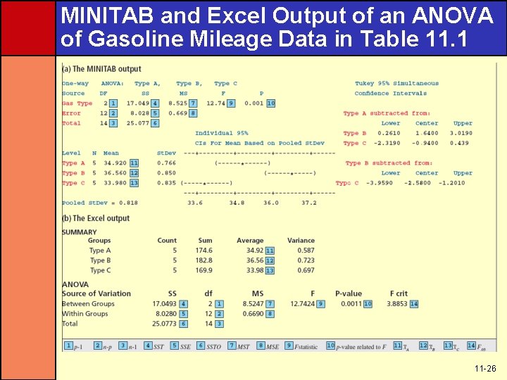
MINITAB and Excel Output of an ANOVA of Gasoline Mileage Data in Table 11. 1 11 -26

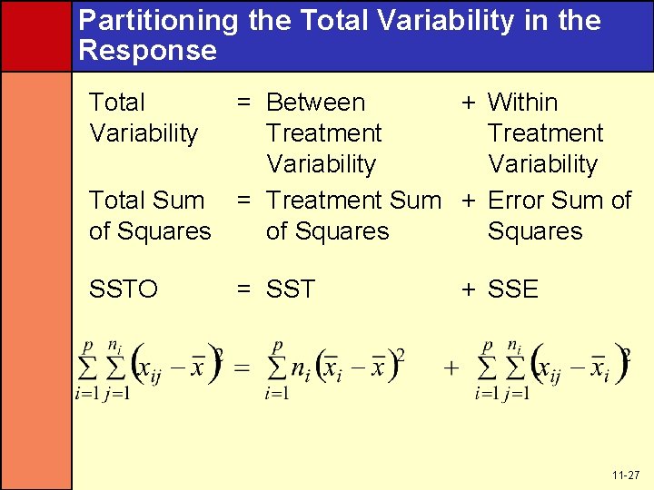
Partitioning the Total Variability in the Response Total Variability = Between + Within Treatment Variability Total Sum = Treatment Sum + Error Sum of of Squares SSTO = SST + SSE 11 -27

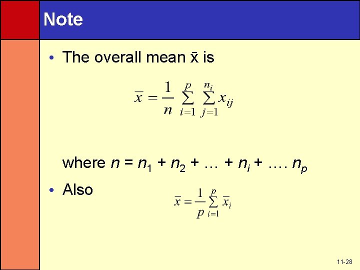
Note • The overall mean x is where n = n 1 + n 2 + … + ni + …. np • Also 11 -28

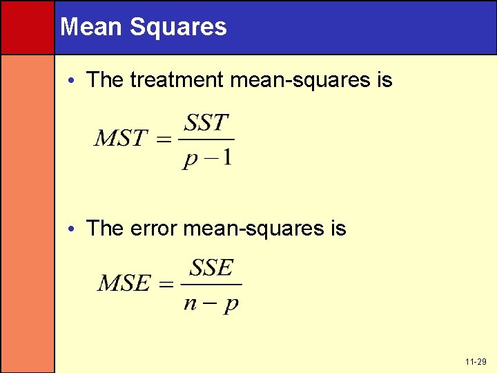
Mean Squares • The treatment mean-squares is • The error mean-squares is 11 -29

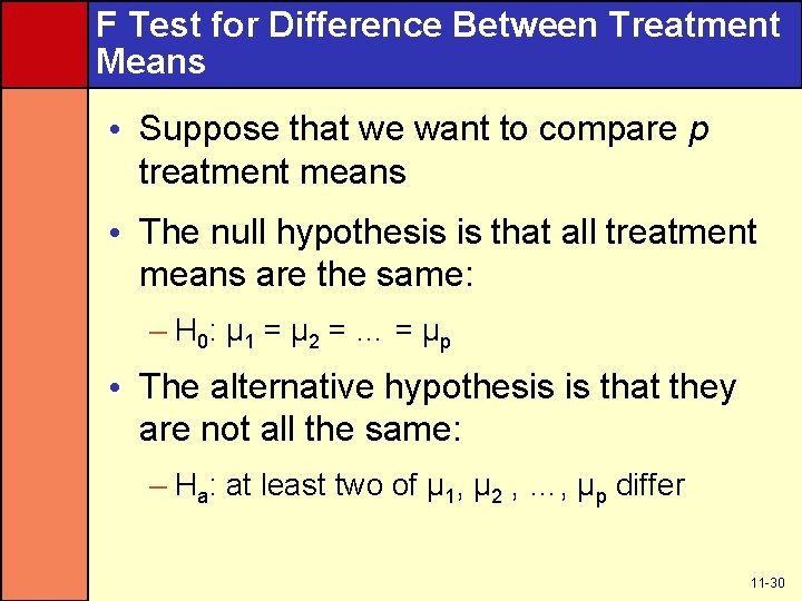
F Test for Difference Between Treatment Means • Suppose that we want to compare p treatment means • The null hypothesis is that all treatment means are the same: – H 0: µ 1 = µ 2 = … = µ p • The alternative hypothesis is that they are not all the same: – Ha: at least two of µ 1, µ 2 , …, µp differ 11 -30

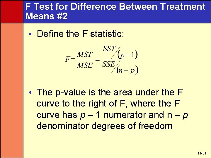
F Test for Difference Between Treatment Means #2 • Define the F statistic: • The p-value is the area under the F curve to the right of F, where the F curve has p – 1 numerator and n – p denominator degrees of freedom 11 -31

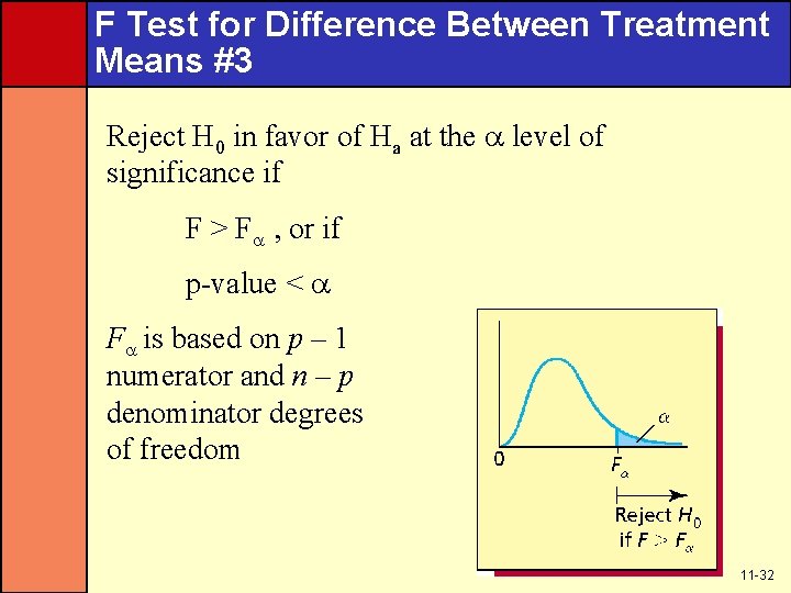
F Test for Difference Between Treatment Means #3 Reject H 0 in favor of Ha at the level of significance if F > F , or if p-value < F is based on p – 1 numerator and n – p denominator degrees of freedom 11 -32

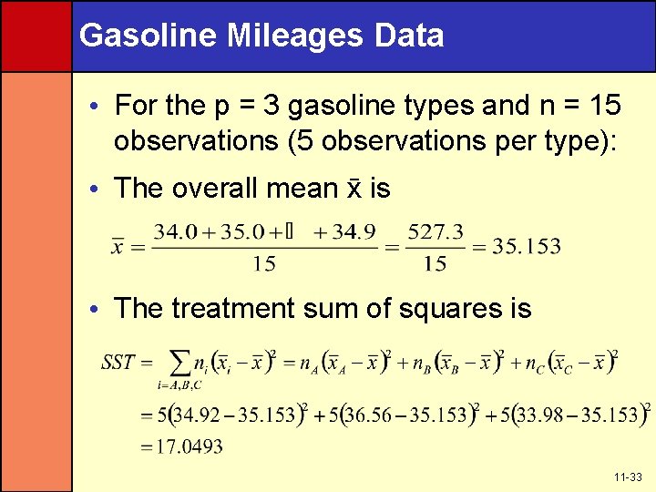
Gasoline Mileages Data • For the p = 3 gasoline types and n = 15 observations (5 observations per type): • The overall mean x is • The treatment sum of squares is 11 -33

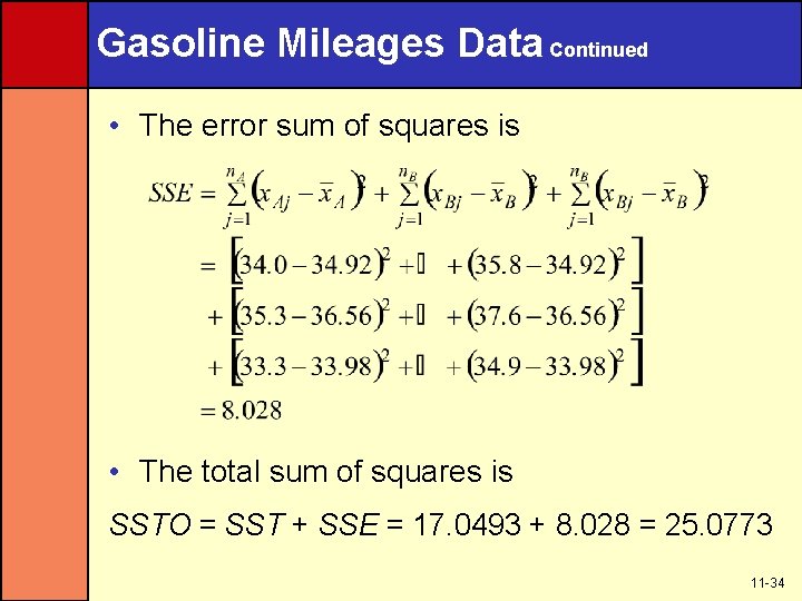
Gasoline Mileages Data Continued • The error sum of squares is • The total sum of squares is SSTO = SST + SSE = 17. 0493 + 8. 028 = 25. 0773 11 -34

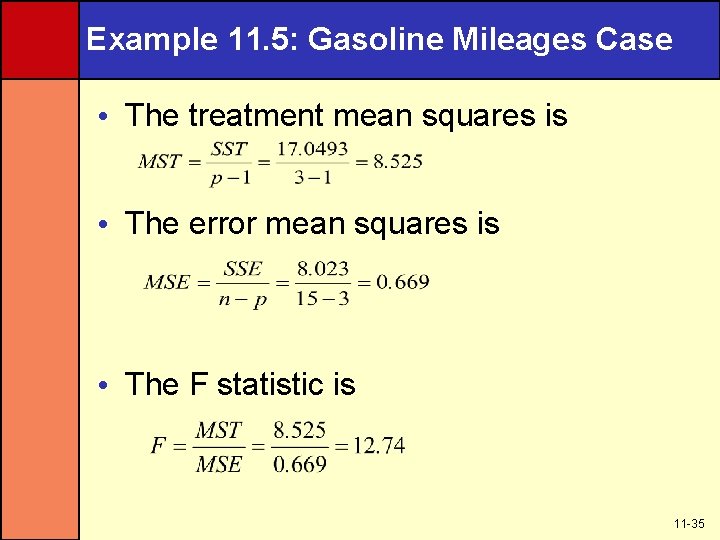
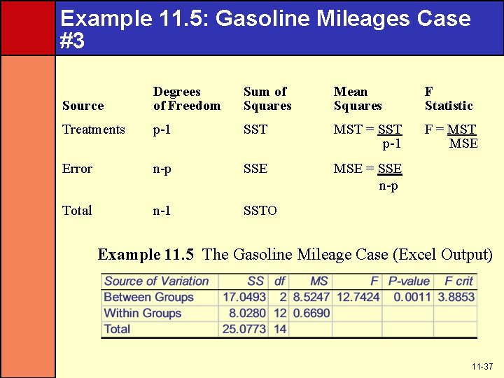
Example 11. 5: Gasoline Mileages Case • The treatment mean squares is • The error mean squares is • The F statistic is 11 -35

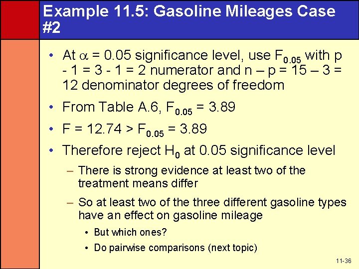
Example 11. 5: Gasoline Mileages Case #2 • At = 0. 05 significance level, use F 0. 05 with p - 1 = 3 - 1 = 2 numerator and n – p = 15 – 3 = 12 denominator degrees of freedom • From Table A. 6, F 0. 05 = 3. 89 • F = 12. 74 > F 0. 05 = 3. 89 • Therefore reject H 0 at 0. 05 significance level – There is strong evidence at least two of the treatment means differ – So at least two of the three different gasoline types have an effect on gasoline mileage • But which ones? • Do pairwise comparisons (next topic) 11 -36

Example 11. 5: Gasoline Mileages Case #3 Source Degrees of Freedom Sum of Squares Mean Squares F Statistic Treatments p-1 SST MST = SST p-1 F = MST MSE Error n-p SSE MSE = SSE n-p Total n-1 SSTO Example 11. 5 The Gasoline Mileage Case (Excel Output) 11 -37

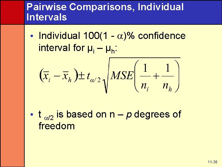
Pairwise Comparisons, Individual Intervals • Individual 100(1 - )% confidence interval for µi – µh: • t /2 is based on n – p degrees of freedom 11 -38

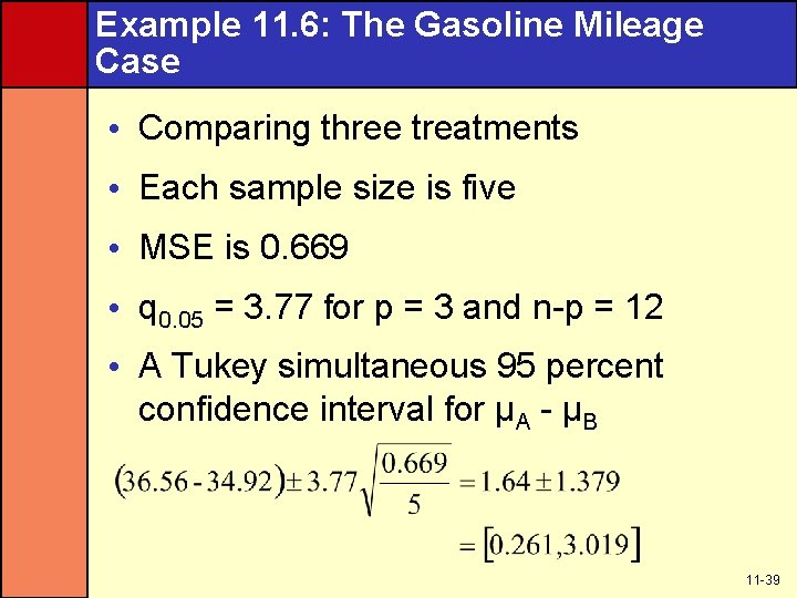
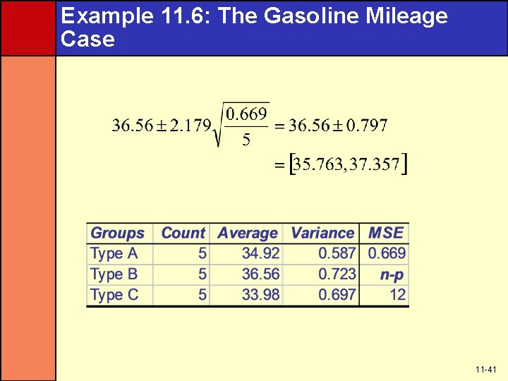
Example 11. 6: The Gasoline Mileage Case • Comparing three treatments • Each sample size is five • MSE is 0. 669 • q 0. 05 = 3. 77 for p = 3 and n-p = 12 • A Tukey simultaneous 95 percent confidence interval for μA - μB 11 -39

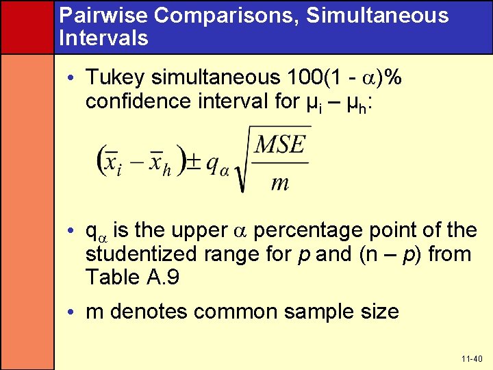
Pairwise Comparisons, Simultaneous Intervals • Tukey simultaneous 100(1 - )% confidence interval for µi – µh: • q is the upper percentage point of the studentized range for p and (n – p) from Table A. 9 • m denotes common sample size 11 -40

Example 11. 6: The Gasoline Mileage Case 11 -41

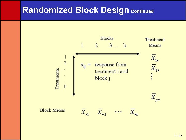
The Randomized Block Design • A randomized block design compares p treatments (for example, production methods) on each of b blocks (or experimental units or sets of units; for example, machine operators) – Each block is used exactly once to measure the effect of each and every treatment – The order in which each treatment is assigned to a block should be random 11 -42

The Randomized Block Design Continued • A generalization of the paired difference design; this design controls for variability in experimental units by comparing each treatment on the same (not independent) experimental units – Differences in the treatments are not hidden by differences in the experimental units (the blocks) 11 -43

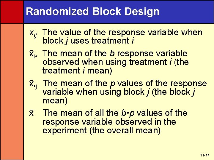
Randomized Block Design xij The value of the response variable when block j uses treatment i xi • The mean of the b response variable observed when using treatment i (the treatment i mean) x • j The mean of the p values of the response variable when using block j (the block j mean) x The mean of all the b • p values of the response variable observed in the experiment (the overall mean) 11 -44

Randomized Block Design Continued 11 -45

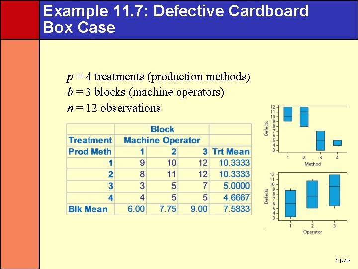
Example 11. 7: Defective Cardboard Box Case p = 4 treatments (production methods) b = 3 blocks (machine operators) n = 12 observations 11 -46

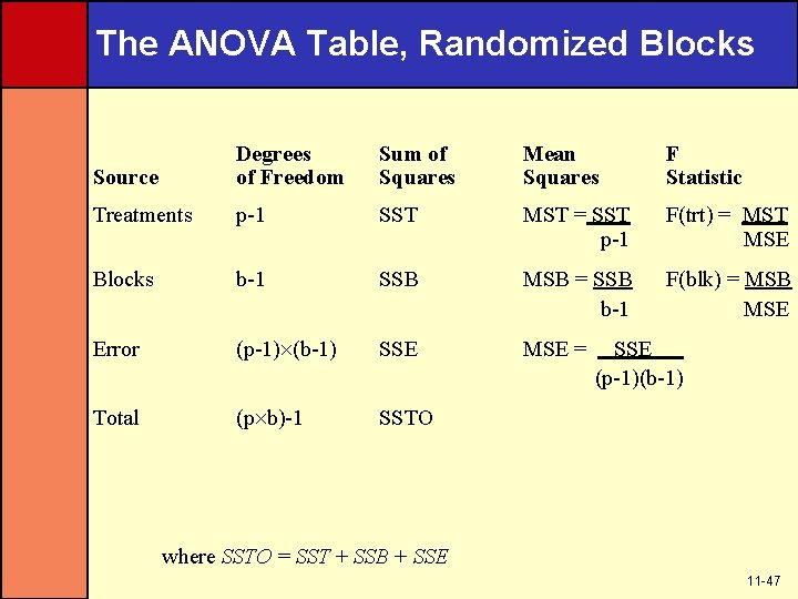
The ANOVA Table, Randomized Blocks Source Degrees of Freedom Sum of Squares Mean Squares F Statistic Treatments p-1 SST MST = SST p-1 F(trt) = MST MSE Blocks b-1 SSB MSB = SSB b-1 F(blk) = MSB MSE Error (p-1) (b-1) SSE MSE = Total (p b)-1 SSTO SSE (p-1)(b-1) where SSTO = SST + SSB + SSE 11 -47

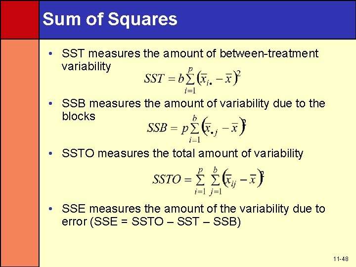
Sum of Squares • SST measures the amount of between-treatment variability • SSB measures the amount of variability due to the blocks • SSTO measures the total amount of variability • SSE measures the amount of the variability due to error (SSE = SSTO – SST – SSB) 11 -48

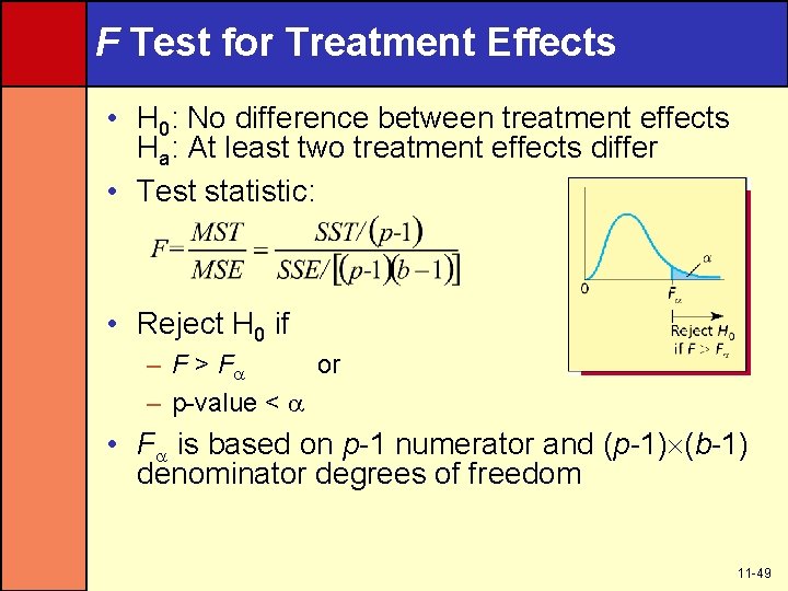
F Test for Treatment Effects • H 0: No difference between treatment effects Ha: At least two treatment effects differ • Test statistic: • Reject H 0 if – F > F or – p-value < • F is based on p-1 numerator and (p-1) (b-1) denominator degrees of freedom 11 -49

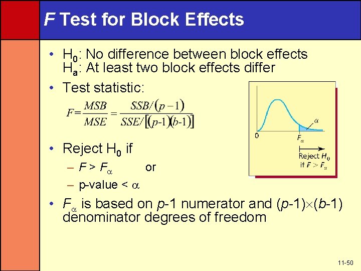
F Test for Block Effects • H 0: No difference between block effects Ha: At least two block effects differ • Test statistic: • Reject H 0 if – F > F or – p-value < • F is based on p-1 numerator and (p-1) (b-1) denominator degrees of freedom 11 -50

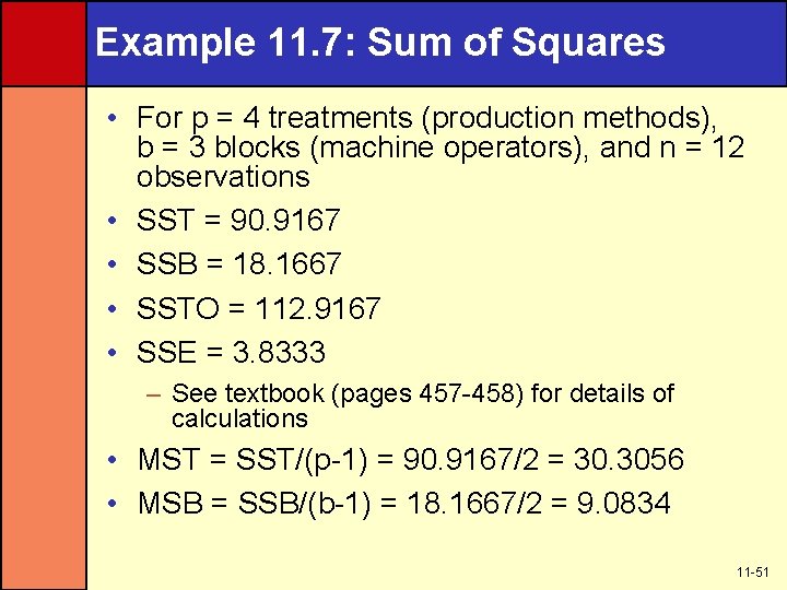
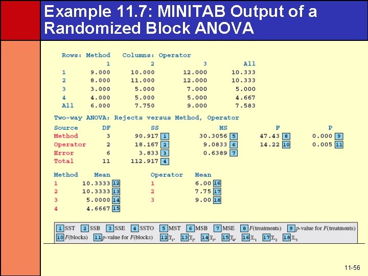
Example 11. 7: Sum of Squares • For p = 4 treatments (production methods), b = 3 blocks (machine operators), and n = 12 observations • SST = 90. 9167 • SSB = 18. 1667 • SSTO = 112. 9167 • SSE = 3. 8333 – See textbook (pages 457 -458) for details of calculations • MST = SST/(p-1) = 90. 9167/2 = 30. 3056 • MSB = SSB/(b-1) = 18. 1667/2 = 9. 0834 11 -51

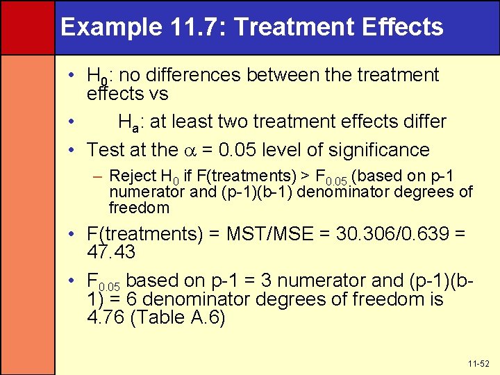
Example 11. 7: Treatment Effects • H 0: no differences between the treatment effects vs • Ha: at least two treatment effects differ • Test at the = 0. 05 level of significance – Reject H 0 if F(treatments) > F 0. 05 (based on p-1 numerator and (p-1)(b-1) denominator degrees of freedom • F(treatments) = MST/MSE = 30. 306/0. 639 = 47. 43 • F 0. 05 based on p-1 = 3 numerator and (p-1)(b 1) = 6 denominator degrees of freedom is 4. 76 (Table A. 6) 11 -52

Example 11. 7: Treatment Effects Continued • F(treatments) = 47. 43 > F 0. 05 = 4. 76 • So reject H 0 at 5% significance level • Therefore, we have strong evidence that at least two production methods (the treatments) have different effects on the mean hourly production of defective boxes 11 -53

Example 11. 7: Block Effects • H 0: no differences between block effects vs Ha: at least two block effects differ • Test at the = 0. 05 level of significance – Reject H 0 if F(blocks) > F 0. 05 (based on p-1 numerator and (p-1)(b-1) denominator degrees of freedom • F(blocks) = MSB/MSE = 9. 083/0. 639 = 14. 22 • F 0. 05 based on b-1 = 2 numerator and (p-1)(b 1) = 6 denominator degrees of freedom is 5. 14 (Table A. 6) 11 -54

Example 11. 7: Block Effects Continued • F(blocks) = 14. 22 > F 0. 05 = 5. 14 • So reject H 0 at 5% significance level • Therefore, we have strong evidence that at least two machine operators (the blocks) have different effects on the mean hourly production of defective boxes 11 -55

Example 11. 7: MINITAB Output of a Randomized Block ANOVA 11 -56

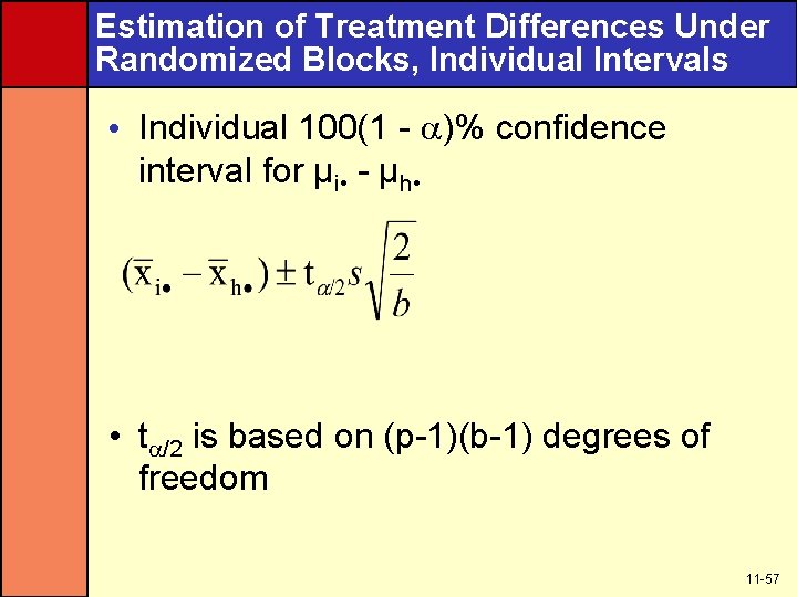
Estimation of Treatment Differences Under Randomized Blocks, Individual Intervals • Individual 100(1 - )% confidence interval for µi • - µh • • t /2 is based on (p-1)(b-1) degrees of freedom 11 -57

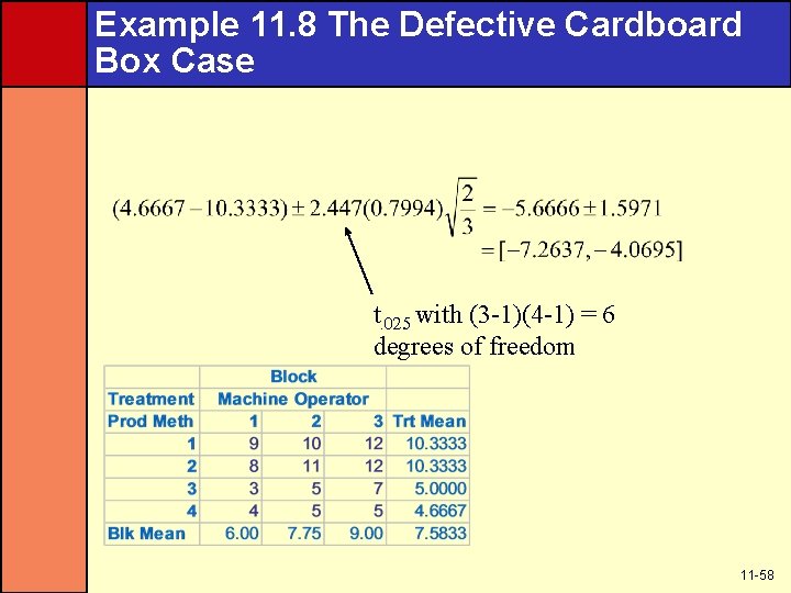
Example 11. 8 The Defective Cardboard Box Case t. 025 with (3 -1)(4 -1) = 6 degrees of freedom 11 -58

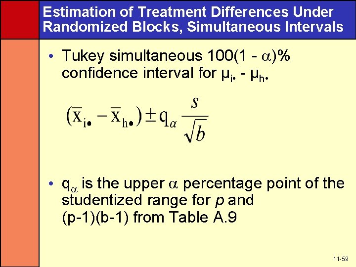
Estimation of Treatment Differences Under Randomized Blocks, Simultaneous Intervals • Tukey simultaneous 100(1 - )% confidence interval for µi • - µh • • q is the upper percentage point of the studentized range for p and (p-1)(b-1) from Table A. 9 11 -59

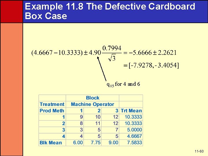
Example 11. 8 The Defective Cardboard Box Case q. 05 for 4 and 6 11 -60

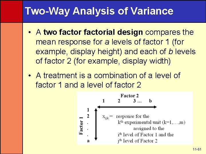
Two-Way Analysis of Variance • A two factorial design compares the mean response for a levels of factor 1 (for example, display height) and each of b levels of factor 2 (for example, display width) • A treatment is a combination of a level of factor 1 and a level of factor 2 11 -61

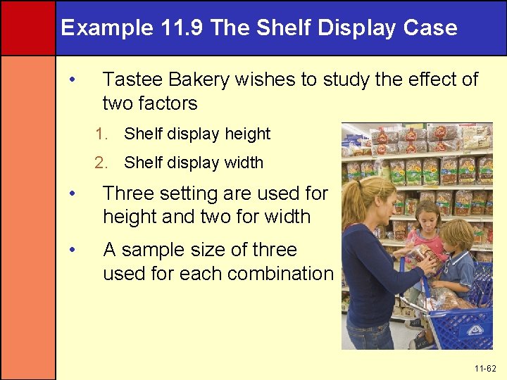
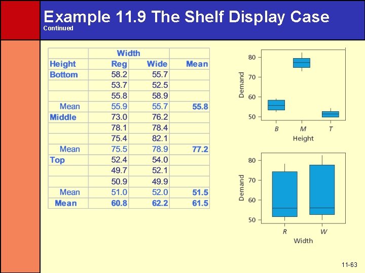
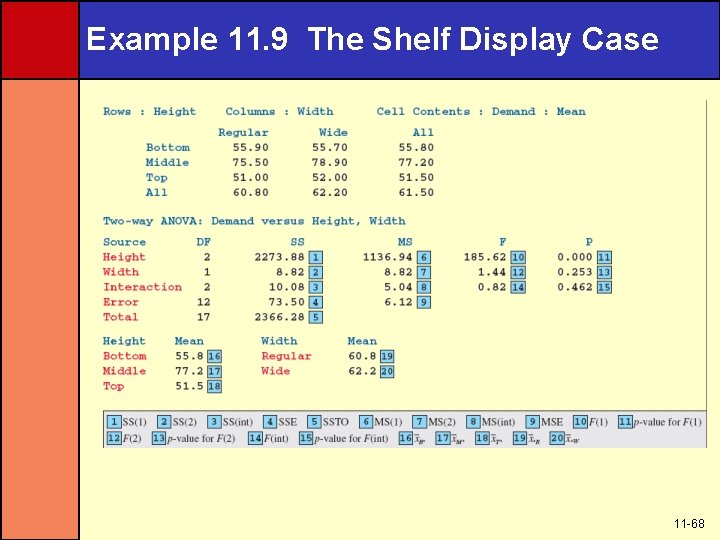
Example 11. 9 The Shelf Display Case • Tastee Bakery wishes to study the effect of two factors 1. Shelf display height 2. Shelf display width • Three setting are used for height and two for width • A sample size of three used for each combination 11 -62

Example 11. 9 The Shelf Display Case Continued 11 -63

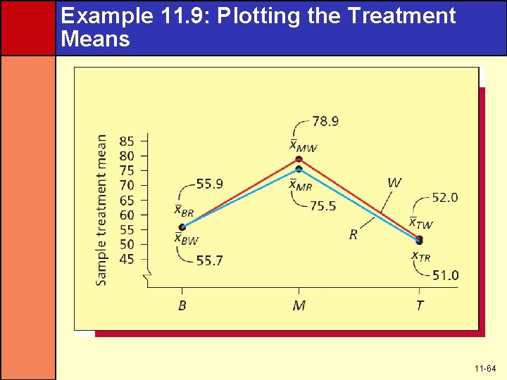
Example 11. 9: Plotting the Treatment Means 11 -64

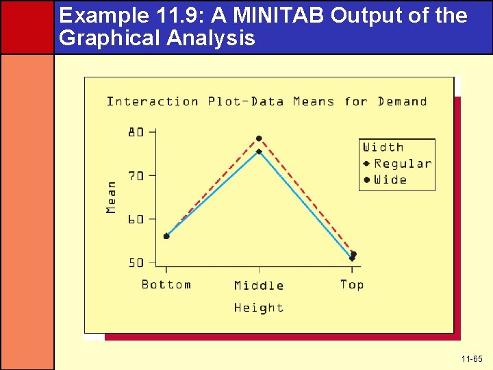
Example 11. 9: A MINITAB Output of the Graphical Analysis 11 -65

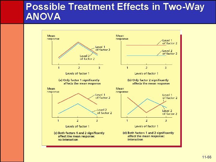
Possible Treatment Effects in Two-Way ANOVA 11 -66

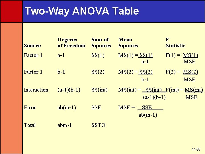
Two-Way ANOVA Table Source Degrees of Freedom Sum of Squares Mean Squares F Statistic Factor 1 a-1 SS(1) MS(1) = SS(1) a-1 F(1) = MS(1) MSE Factor 1 b-1 SS(2) MS(2) = SS(2) b-1 F(2) = MS(2) MSE Interaction (a-1)(b-1) SS(int) MS(int) = SS(int) F(int) = MS(int) (a-1)(b-1) MSE Error ab(m-1) SSE MSE = Total abm-1 SSTO SSE ab(m-1) 11 -67

Example 11. 9 The Shelf Display Case 11 -68

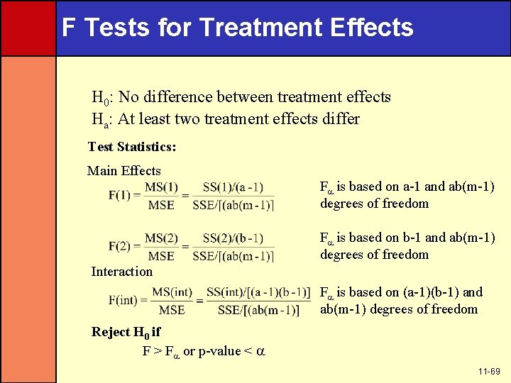
F Tests for Treatment Effects H 0: No difference between treatment effects Ha: At least two treatment effects differ Test Statistics: Main Effects F is based on a-1 and ab(m-1) degrees of freedom F is based on b-1 and ab(m-1) degrees of freedom Interaction F is based on (a-1)(b-1) and ab(m-1) degrees of freedom Reject H 0 if F > F or p-value < 11 -69

Estimation of Treatment Differences Under Two-Way ANOVA, Factor 1 • Individual 100(1 - )% confidence interval for µi • - µi’ • – t /2 is based on ab(m-1) degrees of freedom • Tukey simultaneous 100(1 - )% confidence interval for µi • - µi’ • – q is the upper percentage point of the studentized range for a and ab(m-1) from Table A. 9 11 -70

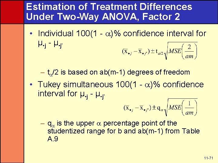
Estimation of Treatment Differences Under Two-Way ANOVA, Factor 2 • Individual 100(1 - )% confidence interval for µ • j - µ • j’ – t /2 is based on ab(m-1) degrees of freedom • Tukey simultaneous 100(1 - )% confidence interval for µ • j - µ • j’ – q is the upper percentage point of the studentized range for b and ab(m-1) from Table A. 9 11 -71