CHAPTER 11 DAC TESTING Basics of Converter Testing

CHAPTER 11 - DAC TESTING

Basics of Converter Testing Intrinsic Parameters Versus Transmission Parameters Chapter 8, “Analog Channel Testing” and Chapter 9, “Sampled Channel Testing”, discussed common channel parameters such as gain, gain tracking, signal to noise ratio (SNR), and signal to distortion ratio (S/D). These parameters are called transmission parameters, or performance parameters, since they describe the effect of the analog or sampled channel on the quality of transmitted signals such as voice or modulated data. In both analog and sampled channels, transmission parameters are determined by the quality of all the channel’s subcircuits

Basics of Converter Testing Intrinsic Parameters Versus Transmission Parameters In this chapter, we will focus on the so called intrinsic parameters of DACs such as absolute error integral non-linearity (INL) and differential non-linearity (DNL). Intrinsic parameters are those parameters that are intrinsic to the circuit itself. They are not dependent on the nature of the test stimulus. © 2015 G. O. Ducoudray

Basics of Converter Testing Intrinsic Parameters Versus Transmission Parameters When testing a DAC or ADC it is common to measure both intrinsic parameters and transmission parameters for full characterization. It is often unnecessary to perform both transmission tests and intrinsic tests in production. Production testing strategy is often determined by the end use of the DAC or ADC Unlike digital circuits which can be tested based on what they are (NAND gate, flip-flop, counter, etc. ), mixed-signal circuits are often tested based on what they do in the system -level application (precision voltage reference, audio signal reconstructor, video signal generator, etc. ). © 2015 G. O. Ducoudray

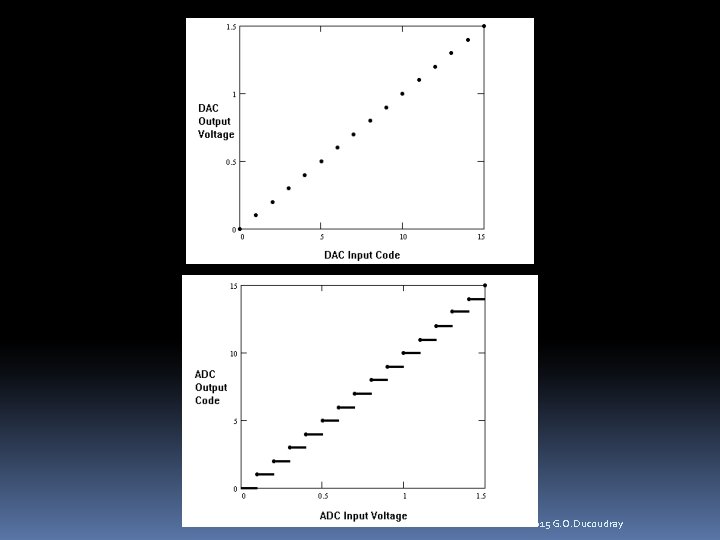
Basics of Converter Testing Comparison of DACs and ADCs Although this chapter is devoted to DAC testing, many DAC concepts are closely tied to ADC testing. For instance, the code-to-voltage transfer characteristics for DACs are similar to the voltage-to-code characteristics of ADCs. It is very important to note that a DAC represents a one-to-one mapping function whereas an ADC represents a many-to-one mapping. For each digital code, a DAC produces only one output voltage. An ADC, by contrast, produces the same output code for a range of input voltages. © 2015 G. O. Ducoudray

Basics of Converter Testing Comparison of DACs and ADCs The difference between DAC and ADC transfer characteristics prevents us from using complementary testing techniques on DACs and ADCs We will concentrate mostly on voltage output DACs. Current output DACs are tested using the same techniques, using either a current mode DC voltmeter or a calibrated voltage-to-current translation circuit located on the device interface board (DIB). © 2015 G. O. Ducoudray

Basics of Converter Testing DAC Failure Mechanisms There are many different types of DACs binary weighted architectures resistive divider architectures pulse width modulated (PWM) architectures pulse density modulated (PDM) architectures (commonly known as Sigma Delta DACs). hybrids of these architectures such as the multi-bit Sigma Delta DAC and segmented resistive divider DACs. Each of these DAC architectures has a unique set of strengths and weaknesses. Each architecture’s weaknesses determine its likely failure mechanisms, and test methodology © 2015 G. O. Ducoudray

Basic DC Tests Code Specific Parameters DAC specifications sometimes require specific voltage levels correspond to specific digital codes Common code-specific parameters include the maximum full scale (+FS) voltage, minimum full scale (-FS) voltage, and midscale (MS) voltage. The midscale voltage typically corresponds to 0 V in bipolar DACs or a center voltage such as Vdd/2 in unipolar (single power supply) DACs. It is important to note that although the minimum full scale voltage is often designated with the –FS notation, it is not necessarily a negative voltage. © 2015 G. O. Ducoudray

Basic DC Tests Full Scale Range Full scale range (FSR) is defined as the voltage difference between the maximum voltage and minimum voltage that can be produced by a DAC. Typically measured by simply measuring the DAC’s +FS voltage, then measuring the DAC’s –FS voltage and subtracting using the equation: FSR = +FS Voltage - -FS Voltage © 2015 G. O. Ducoudray

Basic DC Tests DC Gain, Gain Error, Offset, and Offset Error It is tempting to say that the DAC’s offset is equal to the measured midscale voltage. It is also tempting to define the gain of a DAC as the full scale range divided by the number of spaces, or steps, between codes. These definitions of offset and gain are approximately correct. In fact, they are sometimes defined in spec sheets exactly this way. These definitions would be quite valid in a perfectly linear DAC. However, in an imperfect DAC they are inferior because they are very sensitive to variations in the –FS, MS, and +FS voltage outputs. © 2015 G. O. Ducoudray

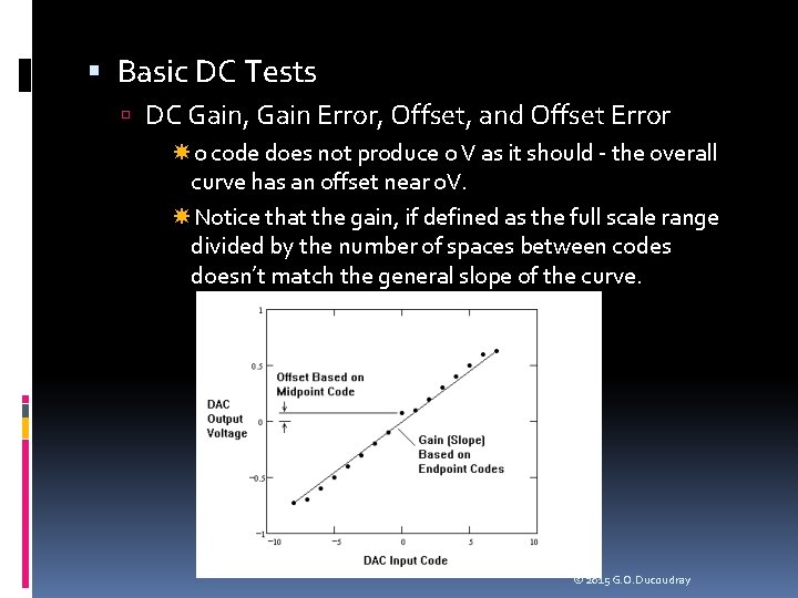
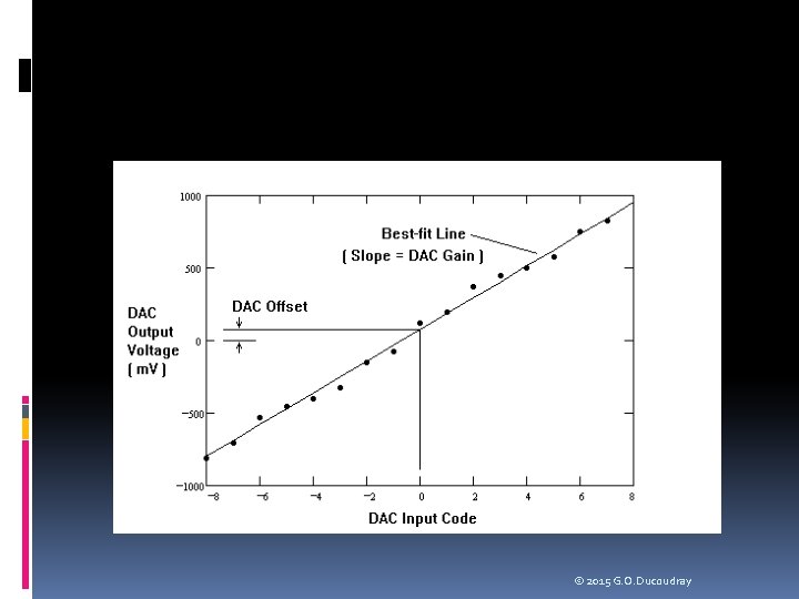
Basic DC Tests DC Gain, Gain Error, Offset, and Offset Error 0 code does not produce 0 V as it should - the overall curve has an offset near 0 V. Notice that the gain, if defined as the full scale range divided by the number of spaces between codes doesn’t match the general slope of the curve. © 2015 G. O. Ducoudray

Basic DC Tests DC Gain, Gain Error, Offset, and Offset Error A less ambiguous definition of gain and offset can be found by computing the best-fit line for these points and then computing the gain and offset of this line. The best-fit line approach is independent of DAC resolution, so it is the preferred technique. A best-fit line is commonly defined as the line having the minimum squared errors between its evenly spaced samples and the actual DAC output samples © 2015 G. O. Ducoudray

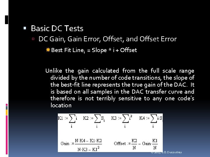
Basic DC Tests DC Gain, Gain Error, Offset, and Offset Error Best Fit Linei = Slope * i + Offset Unlike the gain calculated from the full scale range divided by the number of code transitions, the slope of the best-fit line represents the true gain of the DAC. It is based on all samples in the DAC transfer curve and therefore is not terribly sensitive to any one code’s location © 2015 G. O. Ducoudray

Basic DC Tests DC Gain, Gain Error, Offset, and Offset Error Gain error, expressed as a percent, is defined using the following formula: Gain Error (percent) = 100* ( (Actual Gain / Ideal Gain) – 1) The best-fit line’s calculated offset is not dependent on a single code as it is in the midscale code method. Instead, the best-fit line offset represents the offset of the total sample set. The DAC’s offset is defined as the voltage at which the bestfit line crosses the y-axis. The DAC’s offset error is equal to its offset minus the ideal voltage at this point in the DAC transfer curve © 2015 G. O. Ducoudray

Basic DC Tests LSB Step Size The least significant bit (LSB) step size is defined as the average step size of the DAC transfer curve. It is equal to the gain of the DAC, in volts per bit. It is possible to measure the approximate LSB size by simply dividing the full scale range by the number of code transitions It is more accurate to measure the gain of the best-fit line to calculate the average LSB size © 2015 G. O. Ducoudray

Basic DC Tests DC PSS DAC DC power supply sensitivity (PSS) is easily measured by applying a fixed code to the DAC’s input and measuring the DC gain from one of its power supply pins to its output. PSS for a DAC is therefore identical to the measurement of PSS in any other circuit, as described in Chapter 3. The only difference is that a DAC may have different PSS performance depending on the applied digital code. Usually, a DAC will have the worst PSS performance at its full scale and/or minus full scale settings, because these settings tie the DAC output directly to a voltage derived from the power supply. Worst-case conditions should be used once they have been determined through characterization of the DAC. © 2015 G. O. Ducoudray

Transfer Curve Tests Absolute Error The ideal DAC transfer curve is one in which the step size between each output voltage and the next is exactly equal to the desired LSB step size. Of course, physical DACs don’t behave in an ideal manner, so we have to define figures of merit for their actual transfer curves. One of the simplest figures of merit is the DAC’s maximum and minimum absolute error. An absolute error curve is calculated by subtracting the ideal DAC output curve from the actual measured DAC curve. The values in the absolute error curve can be converted to LSBs by dividing each voltage by the ideal LSB size. The conversion from volts to LSBs is a process called normalization. © 2015 G. O. Ducoudray

Transfer Curve Tests Monotonicity A monotonic DAC is one in which each voltage in the transfer curve is larger than the previous voltage, assuming a rising voltage ramp for increasing codes. If the voltage ramp decreases with increasing code values, we simply have to make sure that each voltage is less than the previous one. Monotonicity testing requires that we take the discrete first derivative of the transfer curve and make sure that each value is positive (for rising ramps) or negative (for falling ramps). The discrete derivative is calculated by simply subtracting each value Si from the next value Si+1. © 2015 G. O. Ducoudray

Transfer Curve Tests Differential Non-Linearity In a perfect DAC, each step would be exactly the ideal LSB step size. Differential non-linearity (DNL) is a figure of merit that describes the uniformity of the LSB step sizes between DAC codes. DNL is also known as differential linearity error (DLE). The DNL curve represents the error in each step size, expressed in fractions of an LSB. DNL is calculated by computing the discrete first derivative of the DACs transfer curve, then normalizing the derivative curve to one LSB, and finally subtracting one LSB from the normalized derivative curve © 2015 G. O. Ducoudray

Transfer Curve Tests Differential Non-Linearity Three basic types of DNL calculations: best-fit, endpoint, and absolute, depending on the method of defining LSB. Best-fit DNL uses the best-fit line’s slope to calculate the average LSB size. Uses gain errors in the DAC without relying on the values of a few individual voltages (best method). Endpoint DNL is calculated by dividing the full scale range by the number of transitions. Depends on the value of the maximum full scale and minimum full scale DAC output levels. highly sensitive to errors in these two values, and is less ideal than the best-fit technique. Finally, the absolute DNL technique uses the ideal LSB size. This technique is not commonly used, since it assumes the DAC’s gain is close to ideal. © 2015 G. O. Ducoudray

Transfer Curve Tests Integral Non-Linearity The integral non-linearity (INL) curve is a comparison between the actual DAC curve and one of three lines: the best-fit line, the endpoint line, or the ideal DAC line. The INL curve, like the DNL curve, is normalized to the LSB step size. As in the DNL case, the best-fit line is the preferred reference line, since it eliminates sensitivity to individual DAC values. © 2015 G. O. Ducoudray

Transfer Curve Tests Integral Non-Linearity The INL curve can be calculated by subtracting the best -fit (or endpoint or ideal) DAC line from the actual DAC curve, dividing the results by the average LSB step size. Note that using the ideal DAC line is equivalent to calculating the absolute error curve. As in DNL testing, we are interested in the maximum and minimum value in the INL curve, which we compare against a limit such as +/- ½ LSB. © 2015 G. O. Ducoudray

Transfer Curve Tests Integral Non-Linearity The INL curve can also be calculated by integrating the DNL curve, thus the term “integral non-linearity”. DNL is a measurement of how consistent the step sizes are from one code to the next. INL is therefore a measure of accumulated errors in the step sizes. Thus, if the DNL values are consistently larger than zero for many codes in a row (step sizes are larger than 1 LSB), the INL curve will exhibit an upward trend. Likewise, if the DNL is less than zero for many codes in a row, the INL curve will exhibit a downward trend. Ideally, the positive error in one code’s DNL will be balanced by negative errors in surrounding codes and vice versa. If this is true, then the INL curve will tend to remain near zero. If not, the INL curve may exhibit large upward or downward bends, causing INL failures. © 2015 G. O. Ducoudray

Transfer Curve Tests Integral Non-Linearity The INL integration is implemented using a running sum of the elements of the DNL. The ith element of the INL curve is equal to the sum of the first i-1 elements of the DNL curve plus a constant of integration. When using the best-fit method, the constant of integration is equal to the difference between the first DAC output voltage and the corresponding point on the best-fit curve. When using the endpoint method, the constant of integration is equal to zero. When using the absolute method, the constant is set to the difference between the first and ideal DAC outputs. In any running sum calculation it is important to use high precision mathematical operations to avoid accumulated error in the running sum. © 2015 G. O. Ducoudray

Transfer Curve Tests Integral Non-Linearity Conversely, DNL can be calculated by taking the first derivative of the INL curve. This is usually the easiest way to calculate DNL when testing DACs, but we will see in the next chapter that the DNL curve for an ADC is easier to capture than the INL curve. In ADC testing it is more common to calculate the DNL curve first, and then integrate it to derive the INL curve. © 2015 G. O. Ducoudray

Problem: A 4 -bit two’s complement DAC produces the following set of voltage levels, starting from code – 8 and progressing through code +7: -780 m. V, -705 m. V, -530 m. V, -455 m. V, -400 m. V, -325 m. V, 150 m. V, -75 m. V, 120 m. V, 195 m. V, 370 m. V, 445 m. V, 500 m. V, 575 m. V, 750 m. V, 825 m. V. These code levels are shown in. Calculate the best-fit line’s gain and offset. The ideal DAC output at code 0 is 0 V. The ideal gain is equal to 100 m. V / bit. Calculate the DAC’s gain (volts per bit), gain error, offset, and offset error. © 2015 G. O. Ducoudray

Solution: We calculate gain and offset resulting in a gain value of 109. 35 m. V / bit and an offset value of – 797. 64 m. V. The gain is equal to 109. 35 m. V and the gain error is given by the equation: Gain Error (%) = 100 * ((109. 35 m. V / 100 m. V) – 1 ) = 9. 35% Because this DAC uses a two’s complement encoding scheme, the offset value is the offset of the best-fit line, not the offset of the DAC. The DAC’s offset is found by calculating the best-fit line’s value at DAC code 0, which corresponds to data point = 8. DAC Offset = 8 * Gain + Offset = 8 * 109. 35 m. V – 797. 64 m. V= 77. 16 m. V DAC Offset Error = DAC Offset – Ideal Offset =77. 16 m. V – 0 V = 77. 16 m. V © 2015 G. O. Ducoudray

Problem: Assuming an ideal gain of 100 m. V per LSB and an ideal offset of 0 V at code 0, calculate the absolute error curve for the 4 -bit DAC of the previous example. Normalize these error values to convert the error curve to LSBs © 2015 G. O. Ducoudray

Solution: The ideal DAC levels are – 800 m. V, -700 m. V, . . . +700 m. V. Subtracting these ideal values from the actual values, we can calculate the absolute voltage errors: +20 m. V, -5 m. V, +70 m. V, +45 m. V, 0 m. V, -25 m. V, +50 m. V, +25 m. V, +120 m. V, +95 m. V, +170 m. V, +145 m. V, +100 m. V, +75 m. V, +150 m. V, +125 m. V. The maximum absolute error is +170 m. V and the minimum absolute error is – 25 m. V. Dividing each value by the ideal LSB size (100 m. V), we get the normalized error curve shown on the next slide. © 2015 G. O. Ducoudray

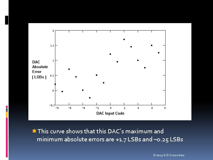
This curve shows that this DAC’s maximum and minimum absolute errors are +1.

Problem: Verify monotonicity in the previous DAC example. Solution: The first derivative of the DAC transfer curve is calculated, yielding the following values: 75 m. V, 175 m. V, 55 m. V, 75 m. V, 175 m. V, 195 m. V, 75 m. V, 175 m. V, 55 m. V, 75 m. V, 175 m. V, 75 m. V Since each value has the same sign (positive), the DAC is monotonic. Notice that there are only 15 first derivative values, even though there are 16 codes in a 4 -bit DAC. This is the nature of the discrete derivative, since there one fewer changes in voltage than there are voltages. © 2015 G. O. Ducoudray

Problem: Calculate the DNL curve for the 4 -bit DAC of the previous examples. Use the best-fit line to define the average LSB size. Does this DAC pass a +/- ½ LSB specification for DNL? © 2015 G. O. Ducoudray

Solution: The first derivative of the transfer curve was calculated in the previous monotonicity example. The first derivative values are: 75 m. V, 175 m. V, 55 m. V, 75 m. V, 175 m. V, 195 m. V, 75 m. V, 175 m. V, 55 m. V, 75 m. V, 175 m. V, 75 m. V. The average LSB size, using the best-fit line calculation was 109. 35 m. V. Dividing each step size by the average LSB size yields the normalized derivative curve (in LSBs): 0. 686, 1. 6, 0. 686, 0. 503, 0. 686, 1. 6, 0. 686, 1. 783, 0. 686, 1. 6, 0. 686, 0. 503, 0. 686, 1. 6, 0. 686. Subtracting one LSB from each of these values gives us the DNL curve for this DAC: -0. 314, 0. 6, -0. 314, -0. 497, -0. 314, 0. 6, 0. 314, 0. 783, -0. 314, 0. 6, -0. 314, -0. 497, -0. 314, 0. 6, -0. 314. © 2015 G. O. Ducoudray

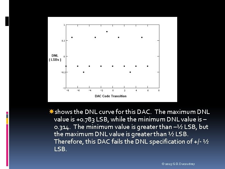
shows the DNL curve for this DAC. The maximum DNL value is +0. 783 LSB, while the minimum DNL value is – 0. 314. The minimum value is greater than –½ LSB, but the maximum DNL value is greater than ½ LSB. Therefore, this DAC fails the DNL specification of +/- ½ LSB. © 2015 G. O. Ducoudray

Problem Calculate the INL curve for the 4 -Bit DAC in the previous examples. First use an endpoint calculation, then use a best-fit calculation. Does either result pass a specification of +/- ½ LSB? Do the two methods produce a significant difference in results? © 2015 G. O. Ducoudray

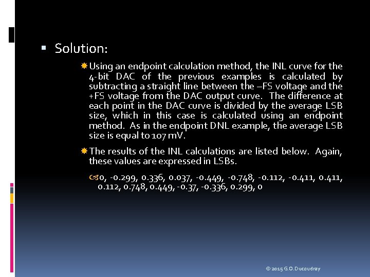
Solution: Using an endpoint calculation method, the INL curve for the 4 -bit DAC of the previous examples is calculated by subtracting a straight line between the –FS voltage and the +FS voltage from the DAC output curve. The difference at each point in the DAC curve is divided by the average LSB size, which in this case is calculated using an endpoint method. As in the endpoint DNL example, the average LSB size is equal to 107 m. V. The results of the INL calculations are listed below. Again, these values are expressed in LSBs. 0, -0. 299, 0. 336, 0. 037, -0. 449, -0. 748, -0. 112, -0. 411, 0. 112, 0. 748, 0. 449, -0. 37, -0. 336, 0. 299, 0 © 2015 G. O. Ducoudray

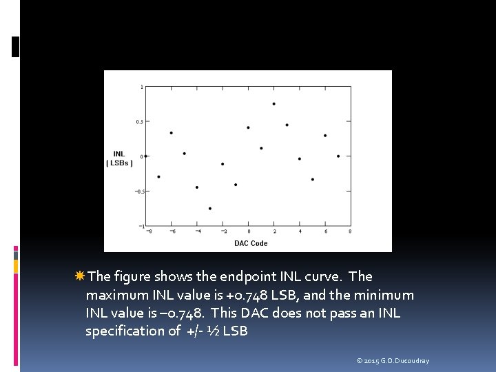
The figure shows the endpoint INL curve. The maximum INL value is +0.

Best Fit Solution Using a best-fit calculation method, the INL curve for the 4 bit DAC of the previous examples is calculated by subtracting the best-fit line from the DAC output curve. Each point in the difference curve is divided by the average LSB size, which in this case is calculated using the best-fit line method. As in the best-fit DNL example, the average LSB size is equal to 109. 35 m. V. The results of the INL calculations are listed below, expressed in LSBs. 0. 161, -0. 153, 0. 448, 0. 133, -0. 364, -0. 678, -0. 077, -0. 392, 0. 077, 0. 678, 0. 364, -0. 133, -0. 448, 0. 153, -0. 161 The best-fit INL curve is shown for comparison with the endpoint INL curve. The maximum value is +0. 678 and the minimum value is – 0. 678. © 2015 G. O. Ducoudray

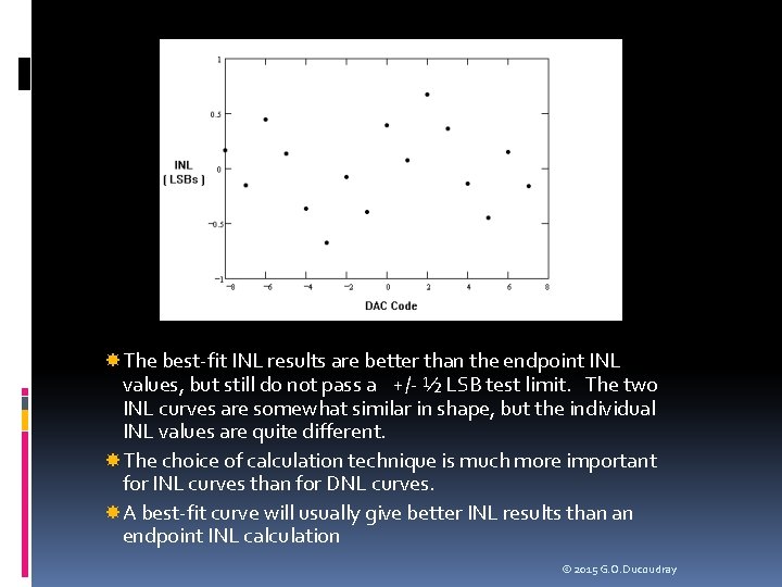
The best-fit INL results are better than the endpoint INL values, but still do not pass a +/- ½ LSB test limit. The two INL curves are somewhat similar in shape, but the individual INL values are quite different. The choice of calculation technique is much more important for INL curves than for DNL curves. A best-fit curve will usually give better INL results than an endpoint INL calculation © 2015 G. O. Ducoudray

Transfer Curve Tests Partial Transfer Curves Nothing prevents a customer or systems engineer from requesting that only a portion of a DAC or ADC transfer curve meet certain specifications. For example, a DAC may be designed so that its –FS code corresponds to 0 V. However, due to analog circuit clipping as the DAC output signal approaches ground, the DAC may clip to a voltage of 100 m. V. If the DAC is designed to perform a specific function that never requires voltages below 100 m. V, then the customer may not care about this clipping. In such a case, the DAC codes below 100 m. V are excluded from the offset, gain, INL, DNL, etc. specifications. © 2015 G. O. Ducoudray

Transfer Curve Tests Major Carrier Testing The techniques discussed thus far for measuring INL and DNL are based on a testing approach called all-codes testing. In allcodes testing, all valid codes in the transfer curve are measured to determine the INL and DNL values. Unfortunately, all-codes testing can be a very time consuming process. Depending on the architecture of the DAC, it may be possible to determine the location of each voltage in the transfer curve without measuring each one explicitly. We will refer to this as selectedcode testing. Selected-code testing can result in significant test time savings, which of course represents a substantial savings in test cost. There are several selected-code testing techniques, the simplest of which is called the major carrier method. © 2015 G. O. Ducoudray

Transfer Curve Tests Major Carrier Testing Many DACs are designed using an architecture in which a series of binary weighted resistors or capacitors are used to convert the individual bits of the converter code into binary weighted currents or voltages. These currents or voltages are summed together to produce the DAC output. For instance, a binary weighted unsigned binary DAC’s output can be described as a sum of binary weighted voltage or current values, W 0, W 1, . . . Wn, multiplied by the individual bits of the DAC’s input code, D 0, D 1, . . . Dn. The DAC’s output value is output = D 0*W 0+D 1*W 1+. . . +Dn*Wn + DC Base where: DAC code bits D 0 -Dn take on the value of 1 or 0; W 1 = 2*W 0; W 2 = 2*W 1 … Wn = 2*Wn-1 DC Base is the DAC output value with a -FS input code © 2015 G. O. Ducoudray

Transfer Curve Tests Major Carrier Testing If this idealized model of the DAC is sufficiently accurate, then we only need to measure the values of W 0, W 1, . . . Wn to predict every voltage in the DACs transfer curve. This DAC testing method is called the major carrier technique. The major carrier approach can be used for ADCs as well as DACs. The assumption of sufficient DAC or ADC model accuracy is only valid if the actual superposition errors of the DAC or ADC are low. The superposition assumption can only be determined through characterization, comparing the all-codes DAC output levels with the ones generated by the major carrier method. © 2015 G. O. Ducoudray

Transfer Curve Tests Major Carrier Testing The most straightforward way to measure the value W 0 is to set DAC code bit D 0 to one and all other bits to zero. Likewise, the other major carrier values Wn can be measured by setting Dn to one and all other bits to zero. However, the resulting output levels are widely different in magnitude. This makes them difficult to measure accurately with a voltmeter, since the voltmeter’s range must be adjusted for each measurement. © 2015 G. O. Ducoudray

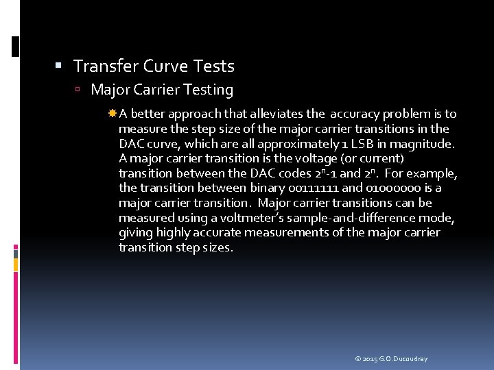
Transfer Curve Tests Major Carrier Testing A better approach that alleviates the accuracy problem is to measure the step size of the major carrier transitions in the DAC curve, which are all approximately 1 LSB in magnitude. A major carrier transition is the voltage (or current) transition between the DAC codes 2 n-1 and 2 n. For example, the transition between binary 00111111 and 01000000 is a major carrier transition. Major carrier transitions can be measured using a voltmeter’s sample-and-difference mode, giving highly accurate measurements of the major carrier transition step sizes. © 2015 G. O. Ducoudray

Transfer Curve Tests Major Carrier Testing Once the step sizes are known, we can use a series of inductive calculations to find the values of W 0, W 1, . . . Wn. We start by realizing that we have actually measured the following values: DC Base = Measured DAC output with minus full scale code V 0 = W 0 V 1 = W 1 – W 0 V 2 = W 2 – (W 1+W 0) V 3 = W 3 – (W 2+W 1+W 0) . . . Vn = Wn – (Wn-1+Wn-2+Wn-3. . . W 0) © 2015 G. O. Ducoudray

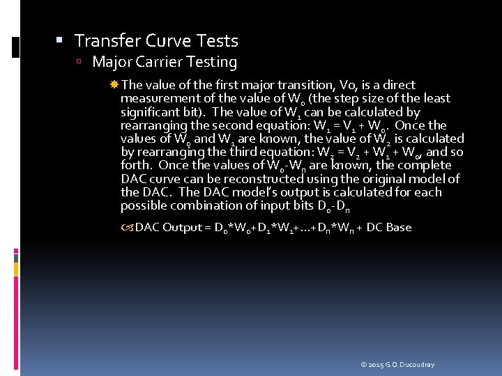
Transfer Curve Tests Major Carrier Testing The value of the first major transition, V 0, is a direct measurement of the value of W 0 (the step size of the least significant bit). The value of W 1 can be calculated by rearranging the second equation: W 1 = V 1 + W 0. Once the values of W 0 and W 1 are known, the value of W 2 is calculated by rearranging the third equation: W 2 = V 2 + W 1 + W 0, and so forth. Once the values of W 0 -Wn are known, the complete DAC curve can be reconstructed using the original model of the DAC. The DAC model’s output is calculated for each possible combination of input bits D 0 -Dn DAC Output = D 0*W 0+D 1*W 1+. . . +Dn*Wn + DC Base © 2015 G. O. Ducoudray

Transfer Curve Tests Major Carrier Testing The major carrier technique can also be used on signed binary and two’s complement converters, although the codes corresponding to the major carrier transitions must be chosen to match the converter encoding scheme. Aside from minor modifications in code selection, the major carrier technique is the same as the simple unsigned binary approach © 2015 G. O. Ducoudray

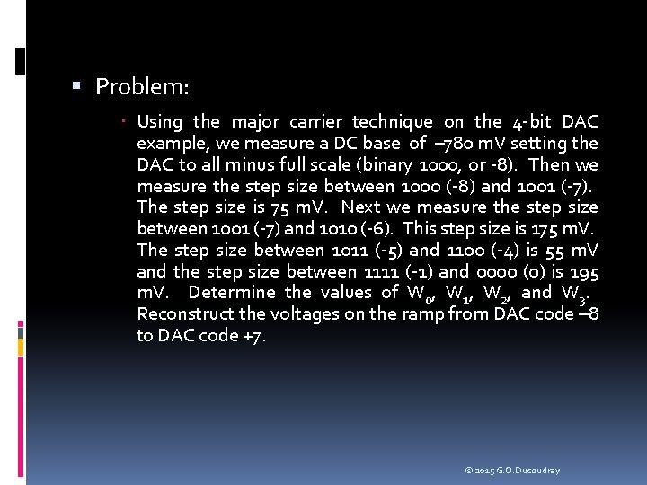
Problem: Using the major carrier technique on the 4 -bit DAC example, we measure a DC base of – 780 m. V setting the DAC to all minus full scale (binary 1000, or -8). Then we measure the step size between 1000 (-8) and 1001 (-7). The step size is 75 m. V. Next we measure the step size between 1001 (-7) and 1010 (-6). This step size is 175 m. V. The step size between 1011 (-5) and 1100 (-4) is 55 m. V and the step size between 1111 (-1) and 0000 (0) is 195 m. V. Determine the values of W 0, W 1, W 2, and W 3. Reconstruct the voltages on the ramp from DAC code – 8 to DAC code +7. © 2015 G. O. Ducoudray

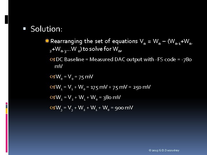
Solution: Rearranging the set of equations Vn = Wn – (Wn-1+Wn 2+Wn-3. . . W 0) to solve for Wn, DC Baseline = Measured DAC output with -FS code = -780 m. V W 0 = V 0 = 75 m. V W 1 = V 1 + W 0 = 175 m. V + 75 m. V = 250 m. V W 2 = V 2 + W 1 + W 0 = 380 m. V W 3 = V 3 + W 2 + W 1 + W 0 = 900 m. V © 2015 G. O. Ducoudray

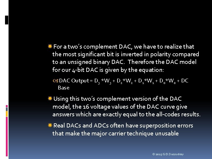
For a two’s complement DAC, we have to realize that the most significant bit is inverted in polarity compared to an unsigned binary DAC. Therefore the DAC model for our 4 -bit DAC is given by the equation: DAC Output = D 3 *W 3 + D 2*W 2 + D 1*W 1 + D 0*W 0 + DC Base Using this two’s complement version of the DAC model, the 16 voltage values of the DAC curve give answers which are exactly equal to the all-codes results. Real DACs and ADCs often have superposition errors that make the major carrier technique unusable © 2015 G. O. Ducoudray

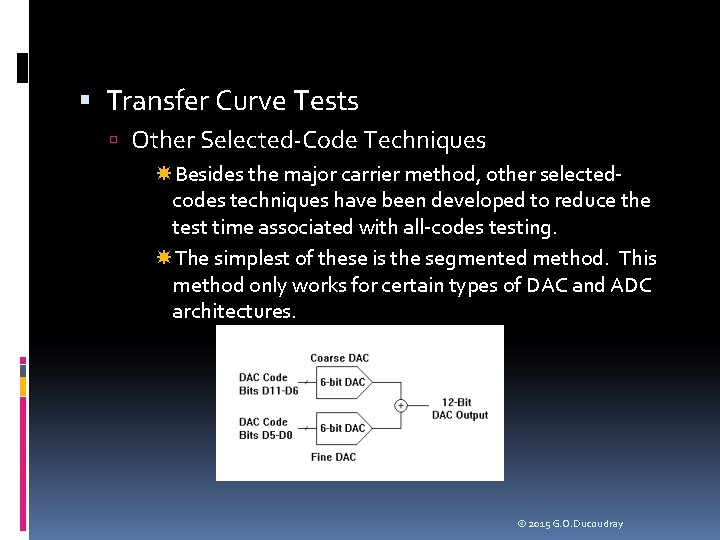
Transfer Curve Tests Other Selected-Code Techniques Besides the major carrier method, other selectedcodes techniques have been developed to reduce the test time associated with all-codes testing. The simplest of these is the segmented method. This method only works for certain types of DAC and ADC architectures. © 2015 G. O. Ducoudray

Transfer Curve Tests Other Selected-Code Techniques NIST technique is based on linear algebra and data collected from production lots to create empirical models of DACs and ADCs. Wavelet transforms to predict overall performance of converters. © 2015 G. O. Ducoudray

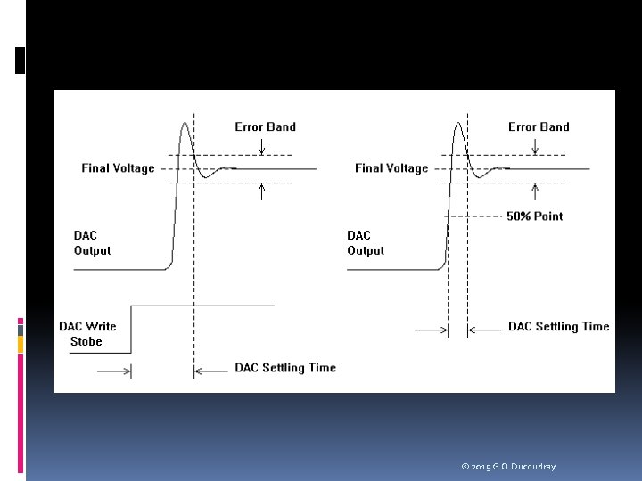
Dynamic DAC Tests Conversion Time (Settling Time) A DAC’s performance is also determined by its dynamic characteristics. One of the most common dynamic tests is settling time, commonly referred to as conversion time. Conversion time is defined as the amount of time it takes for a DAC to stabilize to its final static level within a specified error band after a DAC code has been applied There is one ambiguity in this test. Which DAC code do we start from and which DAC code do we choose as the final destination? The answer is that the DAC must settle from any code to any other code within the specified time. Typically settling time will be measured as the DAC transitions from minus full scale (-FS) to plus full scale (+FS) and vice versa, since these two tests represent the largest voltage swing © 2015 G. O. Ducoudray

Dynamic DAC Tests Conversion Time (Settling Time) The straightforward approach to testing settling time is to digitize the DAC’s output as it transitions from one code to another and then use the known time period between digitizer samples to calculate the settling time. We measure the final settled voltage, calculate the settled voltage limits (i. e. +/- 1/2 LSB) and then calculate the time between the digital signal transition that initiates a DAC code change and the point at which the DAC first stays within the error band limits © 2015 G. O. Ducoudray

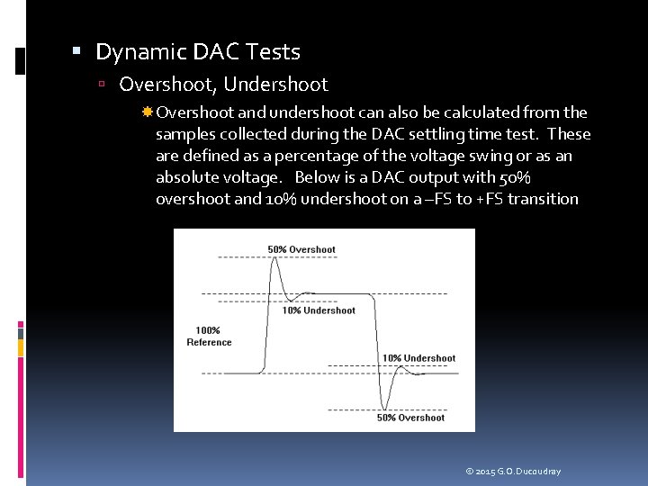
Dynamic DAC Tests Overshoot, Undershoot Overshoot and undershoot can also be calculated from the samples collected during the DAC settling time test. These are defined as a percentage of the voltage swing or as an absolute voltage. Below is a DAC output with 50% overshoot and 10% undershoot on a –FS to +FS transition © 2015 G. O. Ducoudray

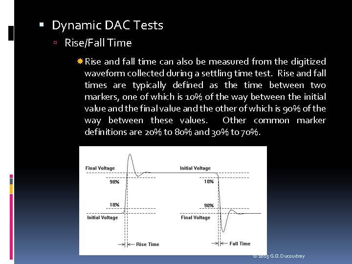
Dynamic DAC Tests Rise/Fall Time Rise and fall time can also be measured from the digitized waveform collected during a settling time test. Rise and fall times are typically defined as the time between two markers, one of which is 10% of the way between the initial value and the final value and the other of which is 90% of the way between these values. Other common marker definitions are 20% to 80% and 30% to 70%. © 2015 G. O. Ducoudray

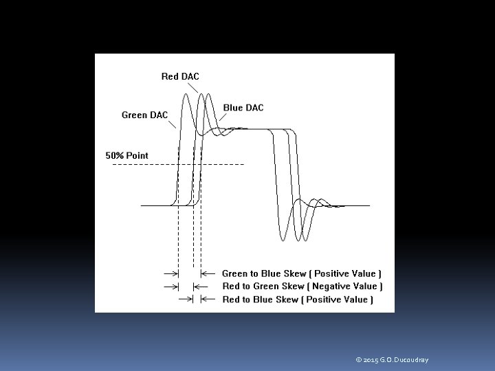
Dynamic DAC Tests DAC to DAC Skew Some types of DACs are designed for use in matched groups. For example, a color palette RAM DAC is a device that is used to produce colors on video monitors. A RAM DAC uses a random access memory (RAM) lookup table to turn a single color value into a set of three DAC output values, representing the red, green, and blue intensity of each pixel. These DAC outputs must change almost simultaneously to produce a clean change from one pixel color to the next. The degree of mismatch between the three DAC outputs is called DAC-to-DAC skew. It is measured by digitizing each DAC output and comparing the timing of the 50% point of each output to the 50% point of the other outputs. There are three skew values (R-G, G-B, and B-R) as illustrated in the next slide. © 2015 G. O. Ducoudray

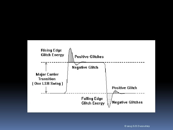
Dynamic DAC Tests Glitch Energy Glitch energy is another specification common to high frequency DACs, especially video DACs. It is defined as the total area of the glitches in a DAC’s output as it transitions across the largest major transition (i. e. 01111111 to 10000000 in an 8 -bit DAC) and back again. These glitches are caused by a combination of capacitive/inductive ringing in the DAC output and skew between the timing of the digital bits feeding the binary weighted DAC circuits. The parameter is expressed in picosecond-volts (ps. V). One area of ambiguity in this specification: is area under the negativegoing spike considered negative area, to be subtracted from the area under the positive spike, or is it positive area to be added? This question should be clarified in the spec sheet to avoid confusion © 2015 G. O. Ducoudray

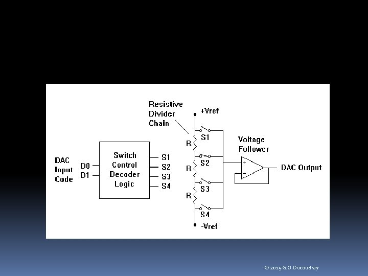
DAC Architectures Resistive Divider DACs Perhaps the simplest DAC architecture is the resistive divider DAC. This type of DAC uses a series-connected string of resistors to produce a set of voltages evenly spaced between +Vref and –Vref. The digital input of the DAC determines which of these voltages is connected through an analog switch to a buffer amplifier. Although the resistive divider architecture may be simple to understand, it quickly loses its appeal for high resolution DACs. Each additional bit of DAC resolution requires twice as many resistors and analog switches. For example, a 12 -bit resistive divider DAC would require 4095 resistors and 4096 switches © 2015 G. O. Ducoudray

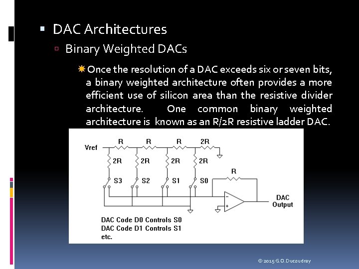
DAC Architectures Binary Weighted DACs Once the resolution of a DAC exceeds six or seven bits, a binary weighted architecture often provides a more efficient use of silicon area than the resistive divider architecture. One common binary weighted architecture is known as an R/2 R resistive ladder DAC. © 2015 G. O. Ducoudray

DAC Architectures Binary Weighted DACs Binary weighted architectures provide two main advantages. First, they are efficient in their use of silicon area. For instance, a 9 -bit current steering DAC only requires one more current source and switch than an 8 -bit current steering DAC. A binary weighted architecture allows major carrier testing, as described earlier, assuming the summation of the individual binary weighted currents or voltages add without superposition error. The major carrier method reduces INL and DNL test time, compared to the brute force all-codes testing method. © 2015 G. O. Ducoudray

DAC Architectures PWM DACs Pulse width modulation (PWM) DACs are very simple DACs that are mostly digital in nature, using very little analog circuitry. PWM DACs adjust their output voltages using a high frequency pulse train of varying duty cycle. The duty cycle controls the amount of time the 1 -bit DAC spends at the VOH level and how much time it spends at the VOL level. Signals are then low pass filtered to create the analog signal. 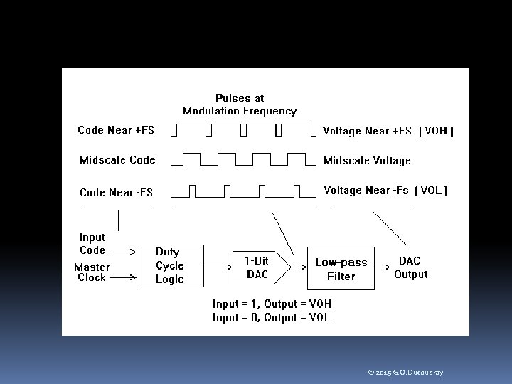© 2015 G. O. Ducoudray

DAC Architectures PWM DACs In many PWM DAC architectures, the duty cycle is produced by purely digital circuits driven by a high frequency master clock. For this reason, the DNL and monotonicity of some PWM DACs are guaranteed by design, as long as the digital logic functions correctly INL, on the other hand, is a potential weakness of all PWM DACs. Depending on the nature of the design architecture. PWM DACs are similar in nature to resistive divider DACs. To obtain a high resolution DAC, a PWM DAC must be able to adjust the pulse train edges by tiny amounts of time. This requires a very high frequency clock to drive the duty cycle generator circuits if a purely digital circuit is to be used. © 2015 G. O. Ducoudray

DAC Architectures PWM DACs One thing in particular limits the resolution of PWM DACs that use purely digital circuits to control pulse widths. Very high resolution DACs require very high frequency master clocks to drive the digital counters controlling the width of the digital pulses (i. e. duty cycle). A 16 -bit PWM DAC, for example, requires a pulse time resolution of 1/65536 th of the period of the pulse train. Since the pulses must be low-pass filtered to generate an analog output, the pulse frequency must be substantially higher (say, a factor of 100) than the highest frequency in the reconstructed analog signal. Therefore, a 16 -bit PWM DAC for audio applications having a 20 k. Hz bandwidth would require a master clock frequency of 65536 times 100 times 20000, or 131 GHz! Clearly, present technology does not support such a design. © 2015 G. O. Ducoudray

DAC Architectures PDM (Sigma Delta) DACs A common solution to this modulation ratio problem is provided by the sigma-delta DAC architecture. Although the digital logic is more complicated than that of a simple PWM DAC, the sigma delta architecture allows a much smaller ratio of master clock to audio bandwidth. A modulation ratio of 50 to 100 allows 16 -bit performance from a sigma delta architecture, compared to a ratio of 6. 5 million to one for a 16 -bit PWM architecture. The sigma delta DAC accomplishes this reduction in master clock frequency using a noise shaping algorithm that moves the quantization noise of the one-bit DAC to high frequencies, cleaning up the low frequency spectrum of the reconstructed signal. © 2015 G. O. Ducoudray

DAC Architectures PDM (Sigma Delta) DACs Sigma delta DACs are well suited for applications requiring relatively low frequency, high quality, AC signal creation. Audio applications such as digital audio and cellular telephony Sigma delta DACs are generally tested for AC parameters such as S/D and SNR rather than the DC transfer curve tests like INL and DNL. In fact, sigma delta DACs are poorly suited to most DC applications because they generate interference signals called self tones. Self tones are low amplitude sinusoidal waves that are generated by the sigma delta noise shaping algorithm itself when certain DC signal levels are applied to the DAC input. © 2015 G. O. Ducoudray

Tests for Common DAC Applications DC References Many DACs are used as simple DC references. An example of this type of DAC usage is the power level control in a cellular telephone. As the cell phone user moves closer or farther away from a cellular base station (the radio antenna tower), the transmitted signal level from the cell phone must be adjusted. The transmitted level is adjusted using a transmit level DAC so that the signal is just strong enough to be received by the base station without draining the cell phone’s battery unnecessarily © 2015 G. O. Ducoudray

Tests for Common DAC Applications DC References AC transmission parameters are probably unimportant. INL and DNL of this DAC would be extremely important, as would its absolute errors, monotonicity, full scale range, and output drive capabilities (output impedance). DACs used as DC references are usually measured using the intrinsic parameters listed in this chapter, rather than the transmission parameters outlined in Chapter 9. © 2015 G. O. Ducoudray

Tests for Common DAC Applications Audio Reconstruction Audio reconstruction DACs are those used to reproduce digitized sound. Examples include the voice-band DAC in a cell phone and the audio DAC in a PC sound card. These DACs are more likely to be tested using transmission parameters, since their purpose is to create audio signals with minimum noise and distortion. The intrinsic parameters such as INL and DNL are often measured for these DACs only during device characterization. Any failures in settling time, glitch energy, etc. , will usually manifest themselves as failures in transmission parameters such as signal to noise, signal to distortion, and idle channel noise. © 2015 G. O. Ducoudray

Tests for Common DAC Applications Data Modulation Data modulation is another purpose to which DACs are often applied. The cellular telephone again provides an example of this type of DAC application. The IF section of a cellular telephone baseband modulator converts digital data into an analog signal suitable for transmission, similar to those used in modems. Like the audio reconstruction DACs, these DACs are typically tested using sine wave or multitone transmission parameter tests. Again, the intrinsic tests like INL and DNL may be added to a characterization test program to help debug the design. However, the intrinsic tests are often removed after the transmission parameters have been verified. Dynamic tests such as settling time may or may not be necessary for data modulation applications © 2015 G. O. Ducoudray

Tests for Common DAC Applications Data Modulation Data modulation DACs also have very specific parameters such as error vector magnitude (EVM) or phase trajectory error (PTE). Parameters such as these are very application-specific. They are usually defined in standards documents published by the IEEE, NIST, or other government or industry organization. The spec sheet should provide references to documents defining application-specific tests such as these. The test engineer is responsible for translating the measurement requirements into ATE-compatible tests that can be performed on a production tester. © 2015 G. O. Ducoudray

Tests for Common DAC Applications Video Signal Generators As discussed earlier, DACs can be used to control the intensity and color of pixels in video CRT displays However, the type of testing required for video DACs depends on the nature of their output. There are two basic types of video DAC applications, RGB and NTSC. RGB (red-green-blue) output is controlled by three separate DACs. Each DAC controls the intensity of an electron beam, which in turn controls the intensity of one of the three primary colors of each pixel as the beam is swept across the CRT tube. In this application, each DAC’s output voltage or current directly control the intensity of the beam. RGB DACs are typically used in computer monitors. © 2015 G. O. Ducoudray

Tests for Common DAC Applications Video Signal Generators The NTSC format is used in transmission of standard analog television signals. It requires only a single DAC, rather than a separate DAC for each color. The picture intensity, color , and saturation information is contained in the offset, amplitude, and phase of a 3. 54 MHz sine wave produced by the DAC. Clearly this is a totally different DAC application than the RGB DAC application. These two seemingly similar video applications require totally different testing approaches. © 2015 G. O. Ducoudray

Tests for Common DAC Applications Video Signal Generators RGB DACs are tested using the standard intrinsic tests like INL and DNL, as well as the dynamic tests like settling time and DAC-to-DAC skew. These parameters are important because the DAC outputs directly control the rapidly changing beam intensities of the red, green, and blue electron beams as they sweep across the computer monitor. Any settling time, rise time, fall time, undershoot, or overshoot, problems show up directly on the monitor as color or intensity distortions, vertical lines, ghost images, etc. The quality of the NTSC video DAC, by contrast, is determined by its ability to produce accurate amplitude and phase shifts in a 3. 54 MHz sine wave, while changing its offset. This type of DAC is tested with transmission parameters like gain, signal to noise, differential gain, and differential phase. © 2015 G. O. Ducoudray

Summary Although DACs all perform the same basic function (digital-to-analog conversion) the architecture of the DAC and its intended application determine its testing requirements and methodologies. A large variety of standard tests have been defined for DACs, including transmission parameters, DC intrinsic parameters, and dynamic parameters. We have to pick and choose DAC test requirements carefully to guarantee the necessary quality of the DAC without wasting time with irrelevant or ineffective tests. © 2015 G. O. Ducoudray

ADDITIONAL PROBLEMS © 2015 G. O. Ducoudray

Problem 8 - 15 Minutes Using the major carrier technique on a 4 -bit DAC, we measure a DC base of -800 m. V setting the DAC to minus full scale (binary 1000 or -8). Then we measure the step size between 1000 and 1001 to be 50 m. V. Next we measure the step size from 1001 to 1010 and obtain 150 m. V. Finally we measure two remaining step transitions (1011 to 1100, giving 55 m. V, and 1111 to 0000 as 190 m. V). Reconstruct the voltages on the ramp from DAC code -8 to DAC code +7 © 2015 G. O. Ducoudray

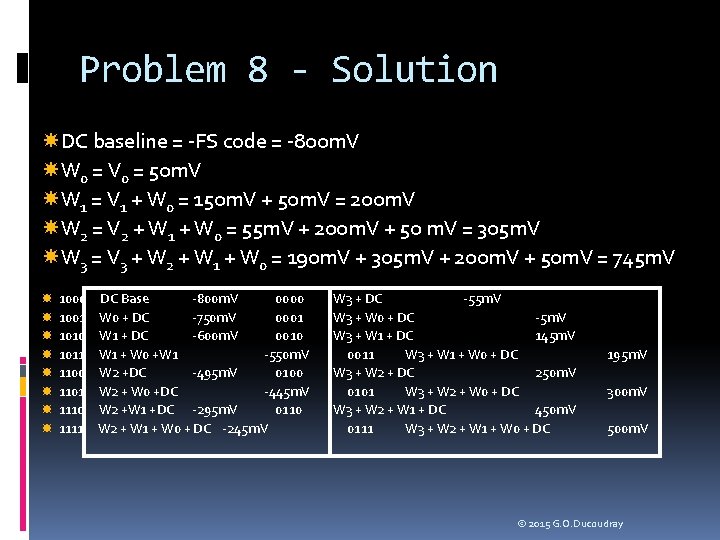
Problem 8 - Solution DC baseline = -FS code = -800 m. V W 0 = V 0 = 50 m. V W 1 = V 1 + W 0 = 150 m. V + 50 m. V = 200 m. V W 2 = V 2 + W 1 + W 0 = 55 m. V + 200 m. V + 50 m. V = 305 m. V W 3 = V 3 + W 2 + W 1 + W 0 = 190 m. V + 305 m. V + 200 m. V + 50 m. V = 745 m. V 1000 1001 1010 1011 1100 1101 1110 1111 DC Base -800 m. V 0000 W 0 + DC -750 m. V 0001 W 1 + DC -600 m. V 0010 W 1 + W 0 +W 1 -550 m. V W 2 +DC -495 m. V 0100 W 2 + W 0 +DC -445 m. V W 2 +W 1 +DC -295 m. V 0110 W 2 + W 1 + W 0 + DC -245 m. V W 3 + DC -55 m. V W 3 + W 0 + DC -5 m. V W 3 + W 1 + DC 145 m. V 0011 W 3 + W 1 + W 0 + DC W 3 + W 2 + DC 250 m. V 0101 W 3 + W 2 + W 0 + DC W 3 + W 2 + W 1 + DC 450 m. V 0111 W 3 + W 2 + W 1 + W 0 + DC 195 m. V 300 m. V 500 m. V © 2015 G. O. Ducoudray

Problem 9 - 10 Minutes From the previous problem, calculate the best -fit line’s gain and offset. The ideal gain and offset are 100 m. V/bit and 0 V at code 0 respectively. Calculate the DAC’s gain, gain error, offset and offset error. © 2015 G. O. Ducoudray

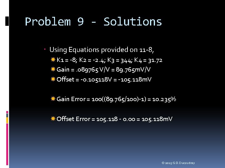
Problem 9 - Solutions Using Equations provided on 11 -8, K 1 = -8; K 2 = -2. 4; K 3 = 344; K 4 = 31. 72 Gain =. 089765 V/V = 89. 765 m. V/V Offset = -0. 105118 V = -105. 118 m. V Gain Error = 100((89. 765/100)-1) = 10. 235% Offset Error = 105. 118 - 0. 00 = 105. 118 m. V © 2015 G. O. Ducoudray

Problem 10 - 15 Minutes From the previous problem, assuming an ideal gain of 100 m. V/bit and an offset of 0 at code 0, calculate the absolute error curve and normalize it to LSB’s © 2015 G. O. Ducoudray

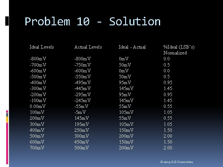
Problem 10 - Solution Ideal Levels Actual Levels Ideal - Actual -800 m. V -700 m. V -600 m. V -500 m. V -400 m. V -300 m. V -200 m. V -100 m. V 0. 00 m. V 100 m. V 200 m. V 300 m. V 400 m. V 500 m. V 600 m. V 700 m. V -800 m. V -750 m. V -600 m. V -550 m. V -495 m. V -445 m. V -295 m. V -245 m. V -5 m. V 145 m. V 195 m. V 250 m. V 300 m. V 450 m. V 500 m. V 50 m. V 95 m. V 145 m. V 55 m. V 105 m. V 150 m. V 200 m. V %Ideal (LSB’s) Normalized 0. 0 0. 5 0. 95 1. 45 0. 55 1. 05 1. 50 2. 00 © 2015 G. O. Ducoudray

Problem 11 - 5 Minutes Verify Monotonicity for the DAC in the previous problems.

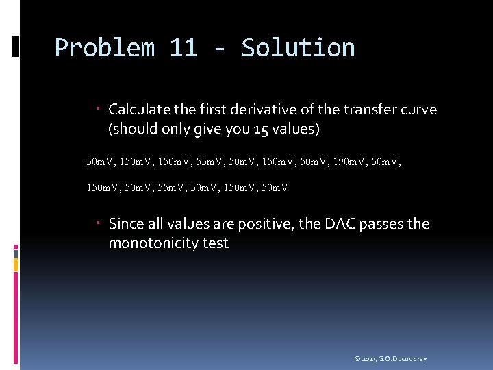
Problem 11 - Solution Calculate the first derivative of the transfer curve (should only give you 15 values) 50 m. V, 150 m. V, 55 m. V, 50 m. V, 150 m. V, 190 m. V, 50 m. V, 150 m. V, 55 m. V, 50 m. V, 150 m. V, 50 m. V Since all values are positive, the DAC passes the monotonicity test © 2015 G. O. Ducoudray

Problem 12 - 15 Minutes Calculate the DNL curve for the 4 bit DAC.

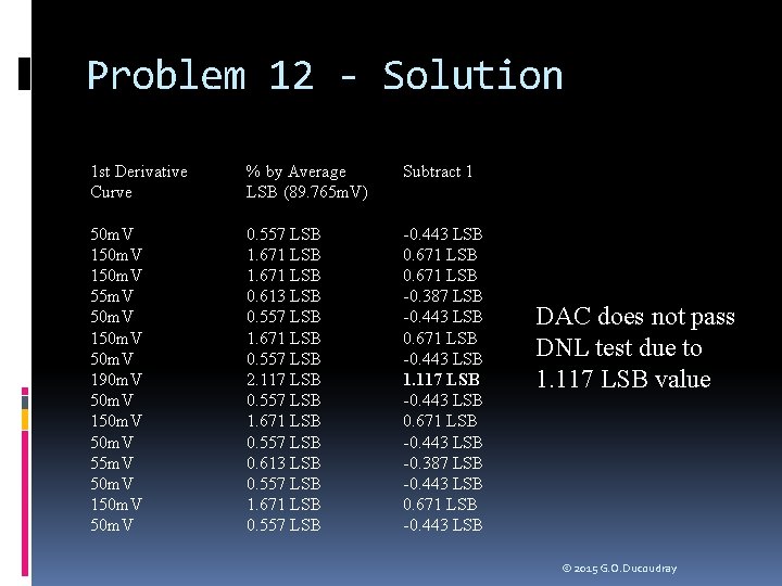
Problem 12 - Solution 1 st Derivative Curve % by Average LSB (89. 765 m. V) Subtract 1 50 m. V 150 m. V 55 m. V 50 m. V 150 m. V 190 m. V 50 m. V 150 m. V 55 m. V 50 m. V 150 m. V 0. 557 LSB 1. 671 LSB 0. 613 LSB 0. 557 LSB 1. 671 LSB 0. 557 LSB 2. 117 LSB 0. 557 LSB 1. 671 LSB 0. 557 LSB 0. 613 LSB 0. 557 LSB 1. 671 LSB 0. 557 LSB -0. 443 LSB 0. 671 LSB -0. 387 LSB -0. 443 LSB 0. 671 LSB -0. 443 LSB 1. 117 LSB -0. 443 LSB 0. 671 LSB -0. 443 LSB -0. 387 LSB -0. 443 LSB 0. 671 LSB -0. 443 LSB DAC does not pass DNL test due to 1. 117 LSB value © 2015 G. O. Ducoudray

Problem 13 - 15 Minutes Using the Best Fit method, calculate the INL of

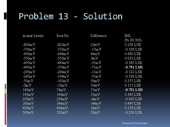
Problem 13 - Solution Actual Levels Best Fit Difference -800 m. V -750 m. V -600 m. V -550 m. V -495 m. V -445 m. V -295 m. V -245 m. V -5 m. V 145 m. V 195 m. V 250 m. V 300 m. V 450 m. V 500 m. V -823 m. V -733 m. V -644 m. V -553 m. V -464 m. V -374 m. V -284 m. V -194 m. V -105 m. V -15 m. V 74 m. V 164 m. V 254 m. V 344 m. V 434 m. V 523 m. V -17 m. V 44 m. V 3 m. V -31 m. V -71 m. V -11 m. V -51 m. V 50 m. V 10 m. V 71 m. V 31 m. V -44 m. V 16 m. V 23 m. V INL (% 89. 765) 0. 256 LSB -0. 189 LSB 0. 490 LSB 0. 033 LSB -0. 345 LSB -0. 791 LSB -0. 122 LSB -0. 568 LSB 0. 557 LSB 0. 111 LSB -0. 791 LSB 0. 345 LSB -0. 045 LSB 0. 490 LSB 0. 178 LSB -0. 256 LSB © 2015 G. O. Ducoudray