Chapter 11 Binomial distribution Analysis of proportion Exact

Chapter 11 Binomial distribution (Analysis of proportion)

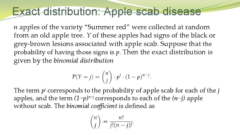
Exact distribution: Apple scab disease n apples of the variety “Summer red” were collected at random from an old apple tree. Y of these apples had signs of the black or grey-brown lesions associated with apple scab. Suppose that the probability of having those signs is p. Then the exact distribution is given by the binomial distribution The term pj corresponds to the probability of apple scab for each of the j apples, and the term (1−p)n−j corresponds to each of the (n−j) apple without scab. The binomial coefficient is defined as

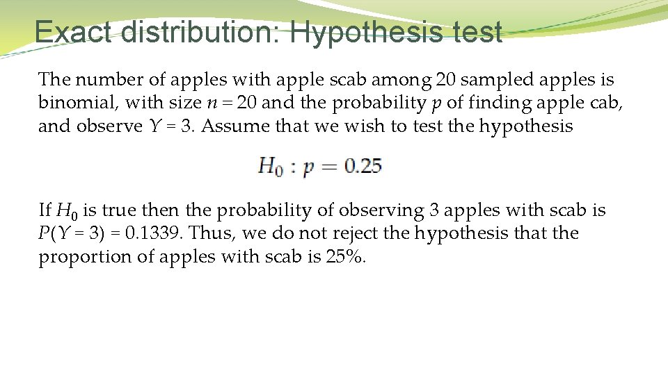
Exact distribution: Hypothesis test The number of apples with apple scab among 20 sampled apples is binomial, with size n = 20 and the probability p of finding apple cab, and observe Y = 3. Assume that we wish to test the hypothesis If H 0 is true then the probability of observing 3 apples with scab is P(Y = 3) = 0. 1339. Thus, we do not reject the hypothesis that the proportion of apples with scab is 25%.

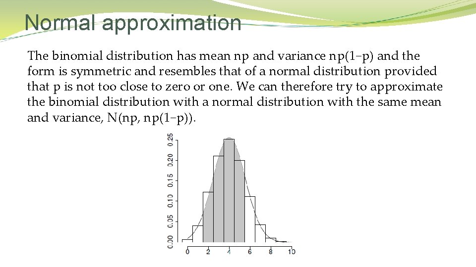
Normal approximation The binomial distribution has mean np and variance np(1−p) and the form is symmetric and resembles that of a normal distribution provided that p is not too close to zero or one. We can therefore try to approximate the binomial distribution with a normal distribution with the same mean and variance, N(np, np(1−p)).

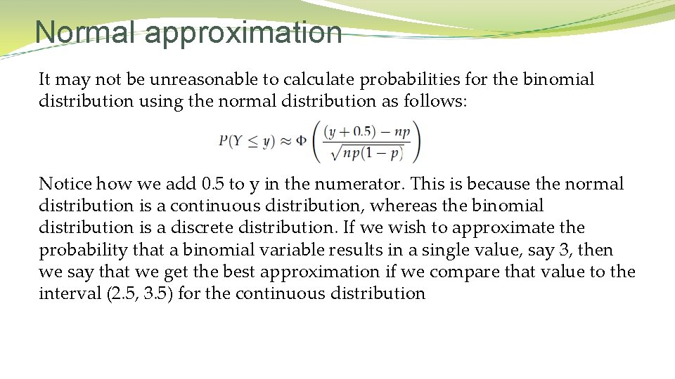
Normal approximation It may not be unreasonable to calculate probabilities for the binomial distribution using the normal distribution as follows: Notice how we add 0. 5 to y in the numerator. This is because the normal distribution is a continuous distribution, whereas the binomial distribution is a discrete distribution. If we wish to approximate the probability that a binomial variable results in a single value, say 3, then we say that we get the best approximation if we compare that value to the interval (2. 5, 3. 5) for the continuous distribution

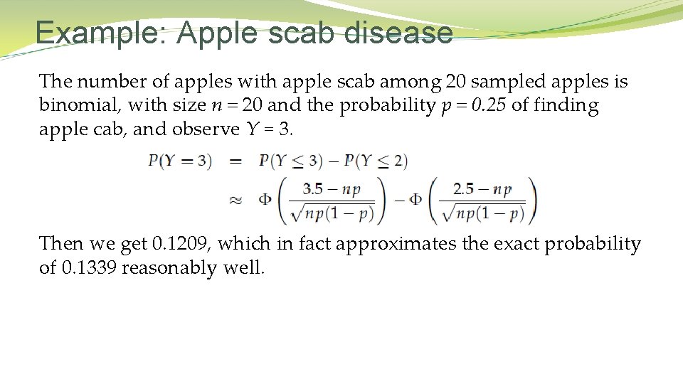
Example: Apple scab disease The number of apples with apple scab among 20 sampled apples is binomial, with size n = 20 and the probability p = 0. 25 of finding apple cab, and observe Y = 3. Then we get 0. 1209, which in fact approximates the exact probability of 0. 1339 reasonably well.

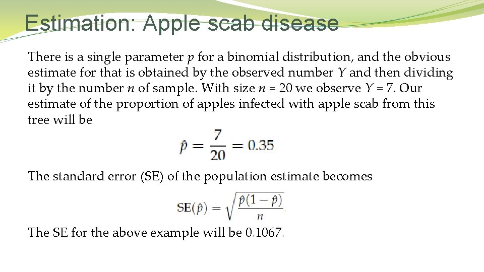
Estimation: Apple scab disease There is a single parameter p for a binomial distribution, and the obvious estimate for that is obtained by the observed number Y and then dividing it by the number n of sample. With size n = 20 we observe Y = 7. Our estimate of the proportion of apples infected with apple scab from this tree will be The standard error (SE) of the population estimate becomes The SE for the above example will be 0. 1067.

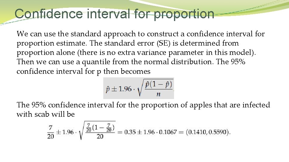
Confidence interval for proportion We can use the standard approach to construct a confidence interval for proportion estimate. The standard error (SE) is determined from proportion alone (there is no extra variance parameter in this model). Then we can use a quantile from the normal distribution. The 95% confidence interval for p then becomes The 95% confidence interval for the proportion of apples that are infected with scab will be

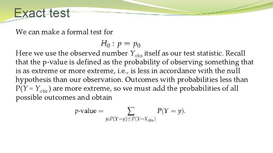
Exact test We can make a formal test for Here we use the observed number Yobs itself as our test statistic. Recall that the p-value is defined as the probability of observing something that is as extreme or more extreme, i. e. , is less in accordance with the null hypothesis than our observation. Outcomes with probabilities less than P(Y = Yobs ) are more extreme, so we must add the probabilities of all possible outcomes and obtain

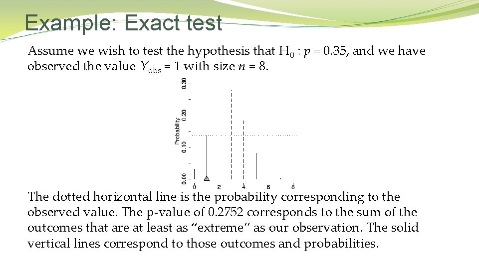
Example: Exact test Assume we wish to test the hypothesis that H 0 : p = 0. 35, and we have observed the value Yobs = 1 with size n = 8. The dotted horizontal line is the probability corresponding to the observed value. The p-value of 0. 2752 corresponds to the sum of the outcomes that are at least as “extreme” as our observation. The solid vertical lines correspond to those outcomes and probabilities.