Chapter 11 Aggregate Supply and the Phillips Curve

Preview • To understand how the economic profession’s views on the Phillips curve evolved

The Phillips Curve • The Phillips curve shows the negative relationship between unemployment and

Policy and Practice: The Phillips Curve Tradeoff and Macroeconomic Policy in the 1960 s

FIGURE 11. 1 Inflation and Unemployment in the United States, 1950 -1969 and 19702009

The Friedman-Phelps Phillips Curve Analysis • Milton Friedman and Edmund Phelps pointed out that

The Friedman-Phelps Phillips Curve Analysis (cont’d) • Their reasoning comes from the expectations-augmented Phillips

The Friedman-Phelps Phillips Curve Analysis (cont’d) • Suppose the unemployment rate is below the

The Friedman-Phelps Phillips Curve Analysis (cont’d) • Conclusions of the Friedman-Phelps Phillips curve analysis:

FIGURE 11. 2 The Short- and Long. Run Phillips Curve Copyright © 2012 Pearson

The Modern Phillips Curve • Given the sharp rise in oil prices in 1973

The Modern Phillips Curve with Adaptive (Backward-Looking) Expectations • How do firms and households

The Modern Phillips Curve with Adaptive (Backward-Looking) Expectations (cont’d) • Substituting in the expectationsaugmented

The Modern Phillips Curve with Adaptive (Backward-Looking) Expectations (cont’d) • The equation is also

The Aggregate Supply Curve • An aggregate supply curve represents the relationship between the

FIGURE 11. 3 Long- and Short-Run Aggregate Supply Curves Copyright © 2012 Pearson Addison-Wesley.

The Short-Run Aggregate Supply Curve • A short-run aggregate supply curve can be derived

FIGURE 11. 4 Okun’s Law, 1960 -2010 Copyright © 2012 Pearson Addison-Wesley. All rights

The Short-Run Aggregate Supply Curve (cont’d) • Substituting in Okun’s law for in the

The Short-Run Aggregate Supply Curve (cont’d) • Numerical example: – Assume $10 trillion –

The Short-Run Aggregate Supply Curve (cont’d) • The short-run Phillips curve implies wages are

Shifts in Aggregate Supply Curves • Shifts in the long-run aggregate supply curve can

FIGURE 11. 5 Shift in the Long-Run Aggregate Supply Curve Copyright © 2012 Pearson

Shifts in the Short-Run Aggregate Supply Curve • Factors that can shift the short-run

FIGURE 11. 6 Shift in the Short-Run Aggregate Supply Curve from Changes in Expected

FIGURE 11. 7 Shift in the Short-Run Aggregate Supply Curve from a Persistent Positive

Slides: 27

Download presentation

Preview • To understand how the economic profession’s views on the Phillips curve evolved over time and how it has affected thinking about macroeconomic policy • To understand how to use the Phillips curve to derive the aggregate supply curve Copyright © 2012 Pearson Addison-Wesley. All rights reserved. 11 -2

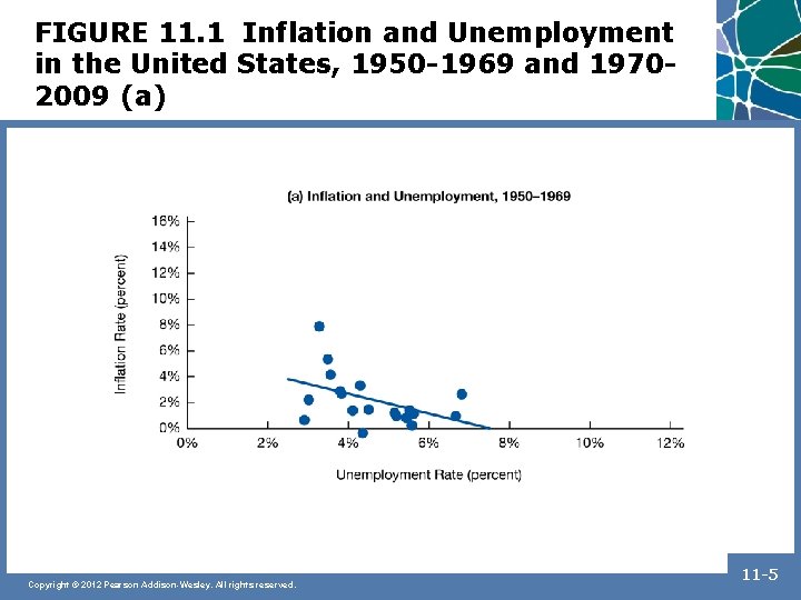
The Phillips Curve • The Phillips curve shows the negative relationship between unemployment and inflation • Named after the New Zealand economist A. W. Phillips for his empirical paper (1958) on the relationship between unemployment and wage growth in the United Kingdom • The Phillips curve seemed to fit the data in the 1960 s very well Copyright © 2012 Pearson Addison-Wesley. All rights reserved. 11 -3

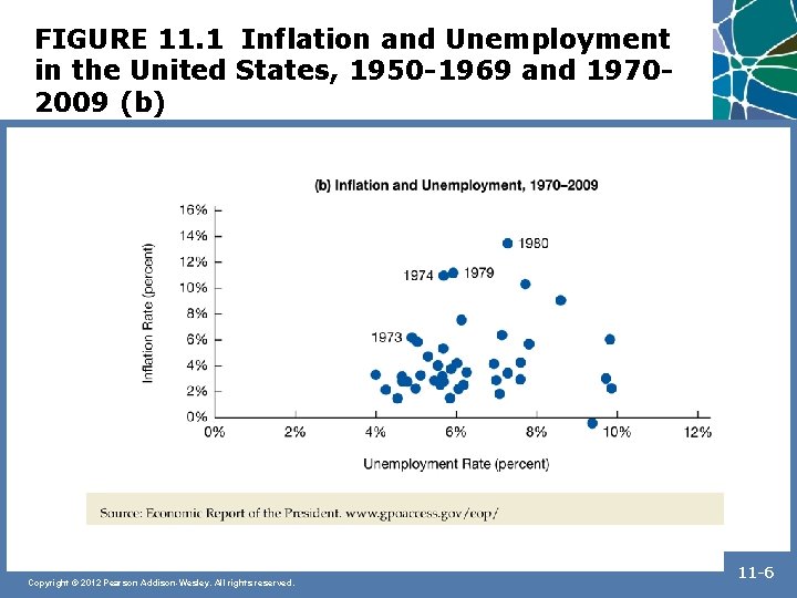
Policy and Practice: The Phillips Curve Tradeoff and Macroeconomic Policy in the 1960 s • In 1960, Paul Samuelson and Robert Solow published a paper outlining how policymakers could exploit the Phillips curve tradeoff between inflation and unemployment • The Kennedy and Johnson administrations followed their advice and pursued expansionary macroeconomic policies that subsequently raised inflation a little bit and brought unemployment down • From the late 1960 s through the 1970 s, however, inflation accelerated while the unemployment rate remained high Copyright © 2012 Pearson Addison-Wesley. All rights reserved. 11 -4

The Friedman-Phelps Phillips Curve Analysis • Milton Friedman and Edmund Phelps pointed out that when all wages and prices were flexible in the long run, the economy would reach the natural rate of unemployment, or the full-employment level of unemployment Copyright © 2012 Pearson Addison-Wesley. All rights reserved. 11 -7

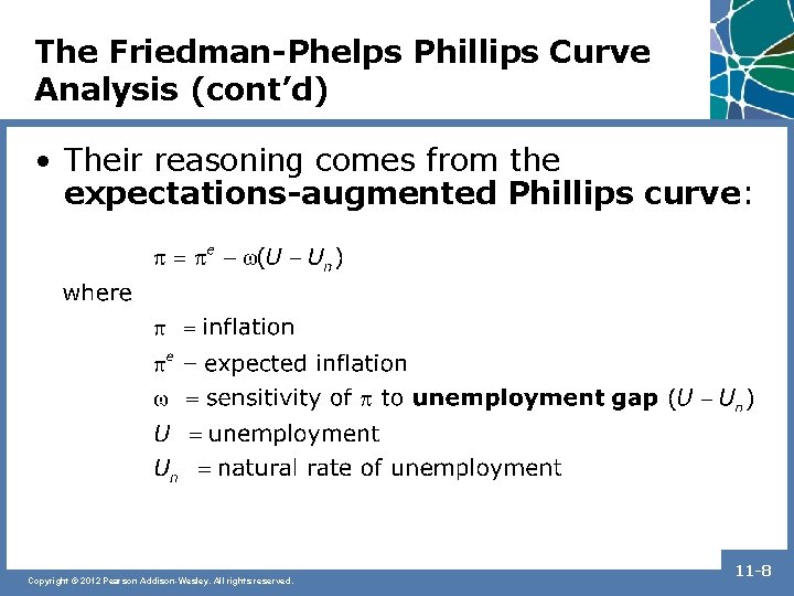
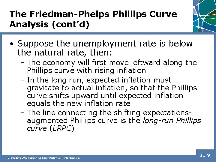
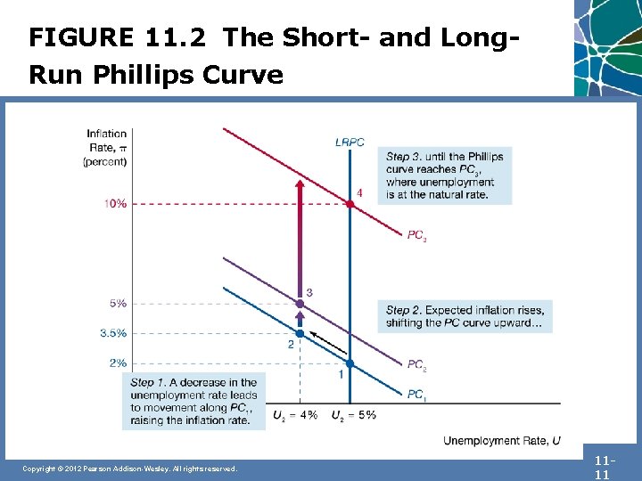
The Friedman-Phelps Phillips Curve Analysis (cont’d) • Suppose the unemployment rate is below the natural rate, then: – The economy will first move leftward along the Phillips curve with rising inflation – In the long run, expected inflation must gravitate to actual inflation, so that the Phillips curve shifts upward until expected inflation equals the new inflation rate – The line connecting the shifting expectationsaugmented Phillips curve is the long-run Phillips curve (LRPC) Copyright © 2012 Pearson Addison-Wesley. All rights reserved. 11 -9

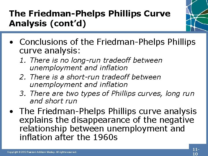
The Friedman-Phelps Phillips Curve Analysis (cont’d) • Conclusions of the Friedman-Phelps Phillips curve analysis: 1. There is no long-run tradeoff between unemployment and inflation 2. There is a short-run tradeoff between unemployment and inflation 3. There are two types of Phillips curves, long run and short run • The Friedman-Phelps Phillips curve analysis explains the disappearance of the negative relationship between unemployment and inflation after the 1960 s Copyright © 2012 Pearson Addison-Wesley. All rights reserved. 1110

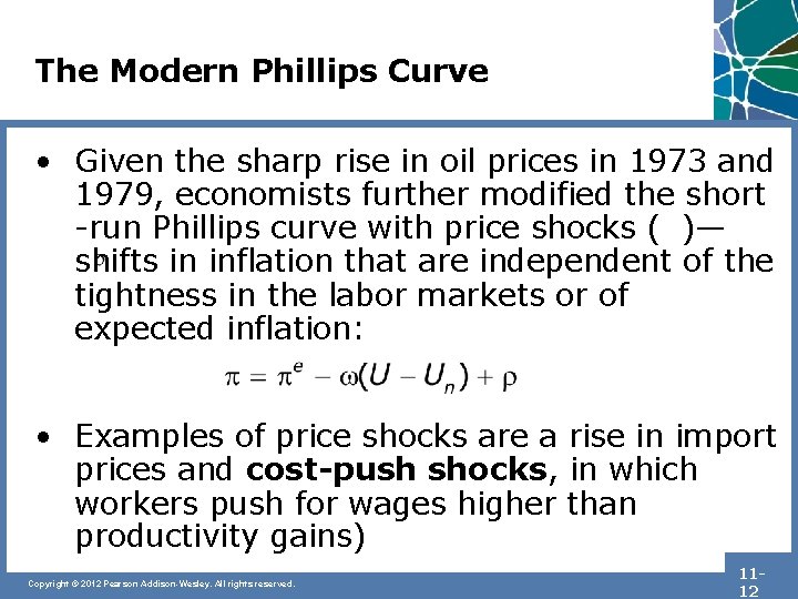
The Modern Phillips Curve • Given the sharp rise in oil prices in 1973 and 1979, economists further modified the short -run Phillips curve with price shocks (_)— shifts in inflation that are independent of the tightness in the labor markets or of expected inflation: • Examples of price shocks are a rise in import prices and cost-push shocks, in which workers push for wages higher than productivity gains) Copyright © 2012 Pearson Addison-Wesley. All rights reserved. 1112

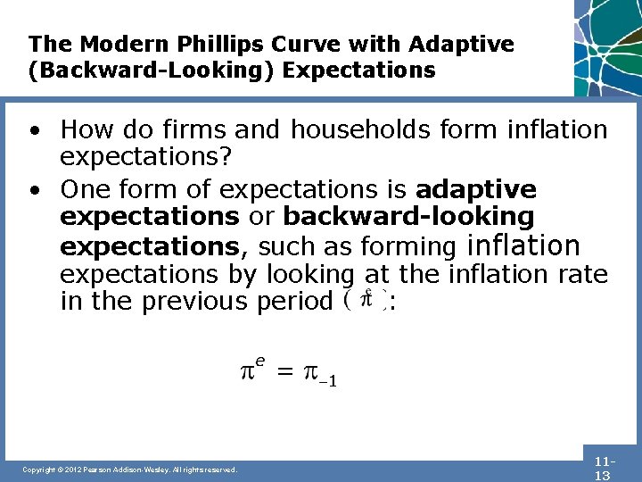
The Modern Phillips Curve with Adaptive (Backward-Looking) Expectations • How do firms and households form inflation expectations? • One form of expectations is adaptive expectations or backward-looking expectations, such as forming inflation expectations by looking at the inflation rate in the previous period : Copyright © 2012 Pearson Addison-Wesley. All rights reserved. 1113

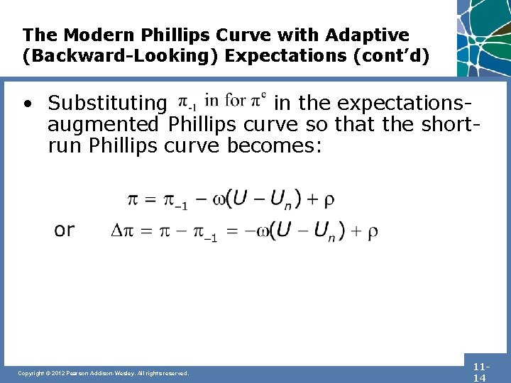
The Modern Phillips Curve with Adaptive (Backward-Looking) Expectations (cont’d) • Substituting in the expectationsaugmented Phillips curve so that the shortrun Phillips curve becomes: Copyright © 2012 Pearson Addison-Wesley. All rights reserved. 1114

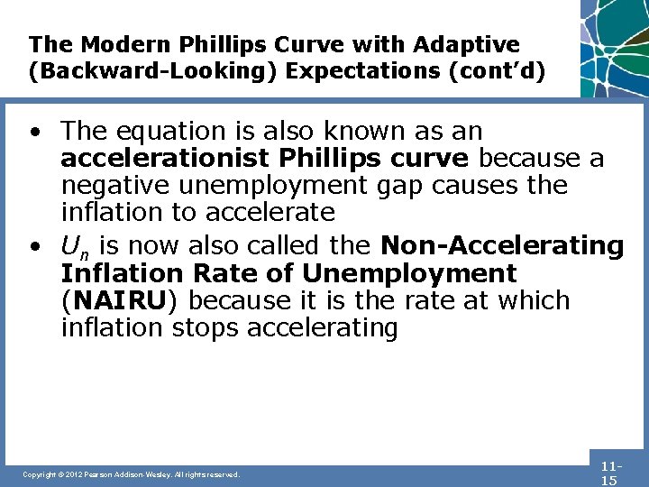
The Modern Phillips Curve with Adaptive (Backward-Looking) Expectations (cont’d) • The equation is also known as an accelerationist Phillips curve because a negative unemployment gap causes the inflation to accelerate • Un is now also called the Non-Accelerating Inflation Rate of Unemployment (NAIRU) because it is the rate at which inflation stops accelerating Copyright © 2012 Pearson Addison-Wesley. All rights reserved. 1115

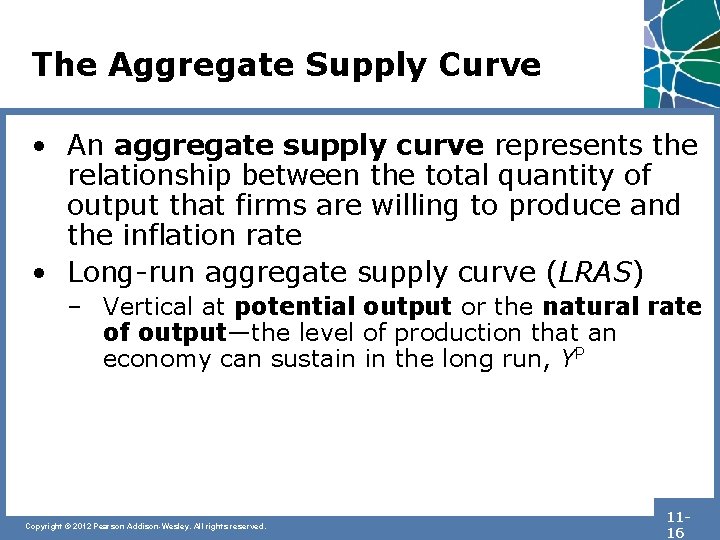
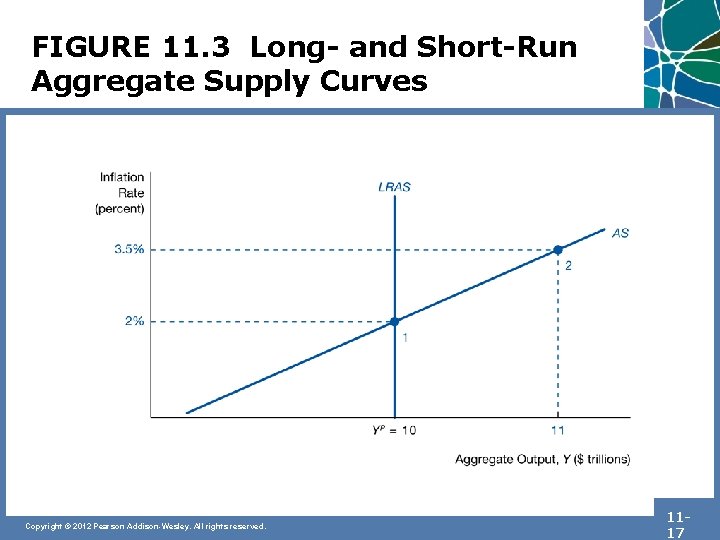
The Aggregate Supply Curve • An aggregate supply curve represents the relationship between the total quantity of output that firms are willing to produce and the inflation rate • Long-run aggregate supply curve (LRAS) – Vertical at potential output or the natural rate of output—the level of production that an economy can sustain in the long run, YP Copyright © 2012 Pearson Addison-Wesley. All rights reserved. 1116

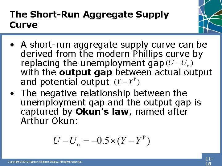
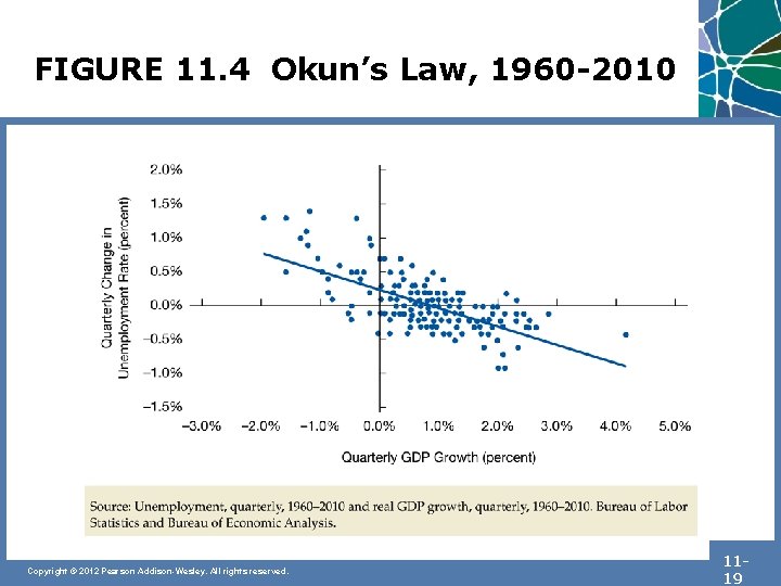
The Short-Run Aggregate Supply Curve • A short-run aggregate supply curve can be derived from the modern Phillips curve by replacing the unemployment gap with the output gap between actual output and potential output • The negative relationship between the unemployment gap and the output gap is captured by Okun’s law, named after Arthur Okun: Copyright © 2012 Pearson Addison-Wesley. All rights reserved. 1118

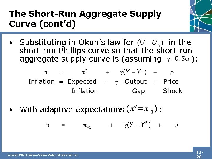
The Short-Run Aggregate Supply Curve (cont’d) • Substituting in Okun’s law for in the short-run Phillips curve so that the short-run aggregate supply curve is (assuming ): • With adaptive expectations Copyright © 2012 Pearson Addison-Wesley. All rights reserved. : 1120

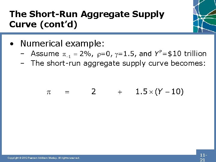
The Short-Run Aggregate Supply Curve (cont’d) • Numerical example: – Assume $10 trillion – The short-run aggregate supply curve becomes: Copyright © 2012 Pearson Addison-Wesley. All rights reserved. 1121

The Short-Run Aggregate Supply Curve (cont’d) • The short-run Phillips curve implies wages are prices are sticky • The short-run aggregate supply curve assumes sticky wages and prices because it is derived from the short-run Phillips curve • The value of indicates the steepness of the short-run aggregate supply curve • When wages and prices are completely flexible, becomes so large that the shortrun aggregate supply curve becomes vertical and so it is identical to the LRAS Copyright © 2012 Pearson Addison-Wesley. All rights reserved. 1122

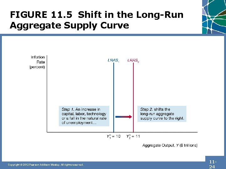
Shifts in Aggregate Supply Curves • Shifts in the long-run aggregate supply curve can come from factors that change potential output (Chapter 3): 1. The total amount of capital 2. The amount of labor supplied 3. The available technology that puts labor and capital together in producing goods and services Copyright © 2012 Pearson Addison-Wesley. All rights reserved. 1123

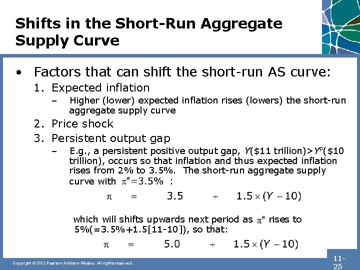
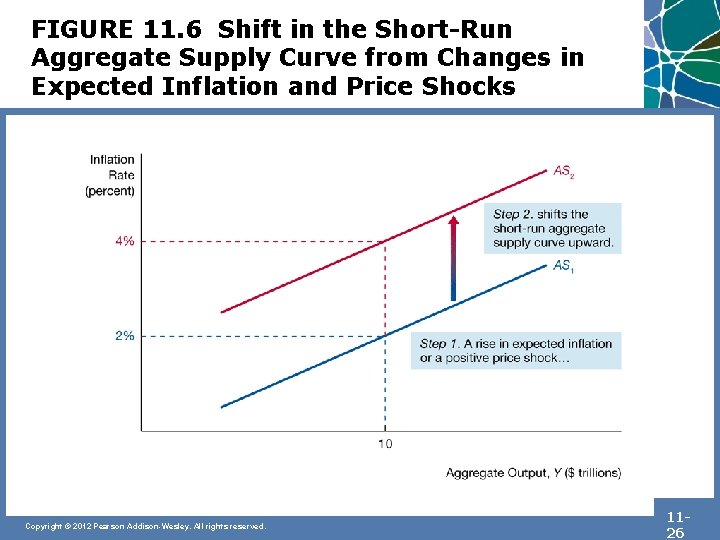
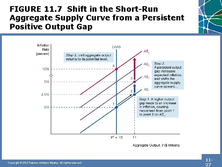
Shifts in the Short-Run Aggregate Supply Curve • Factors that can shift the short-run AS curve: 1. Expected inflation – Higher (lower) expected inflation rises (lowers) the short-run aggregate supply curve 2. Price shock 3. Persistent output gap – E. g. , a persistent positive output gap, Y($11 trillion)>YP($10 trillion), occurs so that inflation and thus expected inflation rises from 2% to 3. 5%. The short-run aggregate supply curve with : which will shifts upwards next period as 5%(=3. 5%+1. 5[11 -10]), so that: Copyright © 2012 Pearson Addison-Wesley. All rights reserved. rises to 1125