Chapter 10 Statistical Inference for Two Samples Learning

Chapter 10 Statistical Inference for Two Samples

Learning Objectives • Comparative experiments involving two samples • Test hypotheses on the difference in means of two normal distributions • Test hypotheses on the ratio of the variances or standard deviations of two normal distributions • Test hypotheses on the difference in two population proportions • Compute power, type II error probability, and make sample size decisions for two-sample tests • Explain and use the relationship between confidence intervals and hypothesis tests

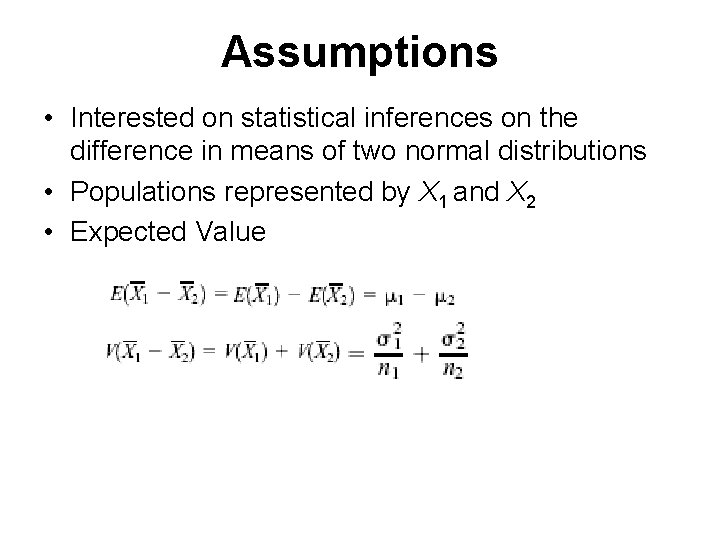
Assumptions • Interested on statistical inferences on the difference in means of two normal distributions • Populations represented by X 1 and X 2 • Expected Value

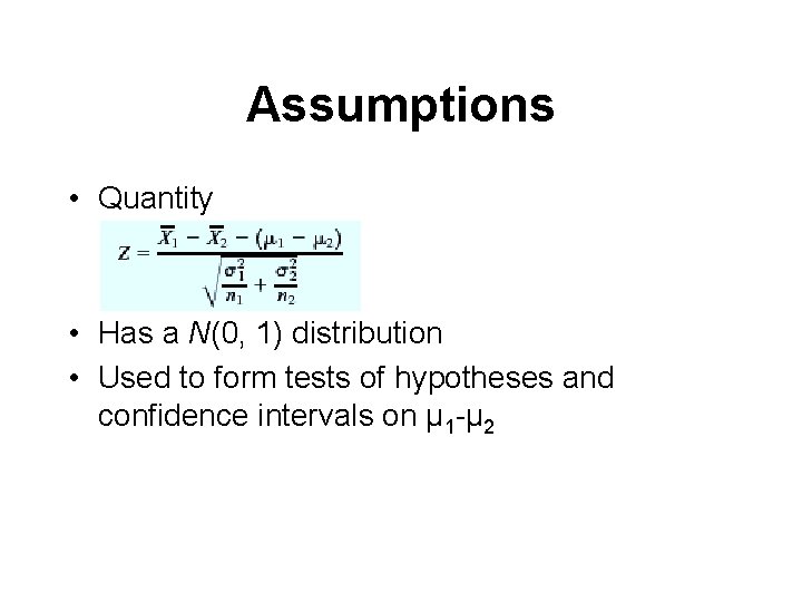
Assumptions • Quantity • Has a N(0, 1) distribution • Used to form tests of hypotheses and confidence intervals on μ 1 -μ 2

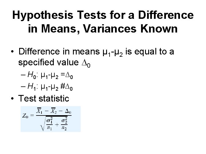
Hypothesis Tests for a Difference in Means, Variances Known • Difference in means μ 1 -μ 2 is equal to a specified value ∆0 – H 0: μ 1 -μ 2 =∆0 – H 1: μ 1 -μ 2 #∆0 • Test statistic

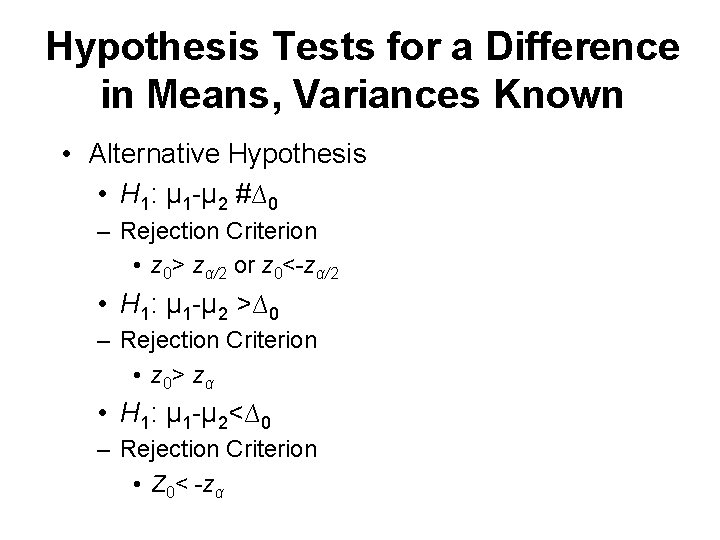
Hypothesis Tests for a Difference in Means, Variances Known • Alternative Hypothesis • H 1: μ 1 -μ 2 #∆0 – Rejection Criterion • z 0> zα/2 or z 0<-zα/2 • H 1: μ 1 -μ 2 >∆0 – Rejection Criterion • z 0> zα • H 1: μ 1 -μ 2<∆0 – Rejection Criterion • Z 0< -zα

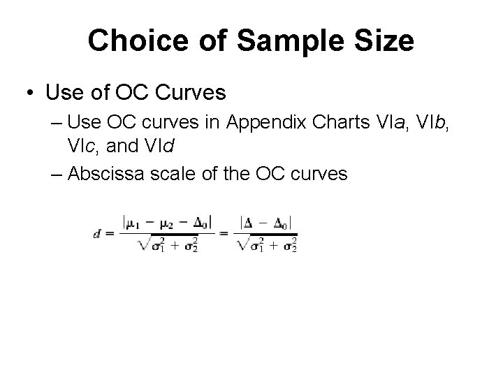
Choice of Sample Size • Use of OC Curves – Use OC curves in Appendix Charts VIa, VIb, VIc, and VId – Abscissa scale of the OC curves

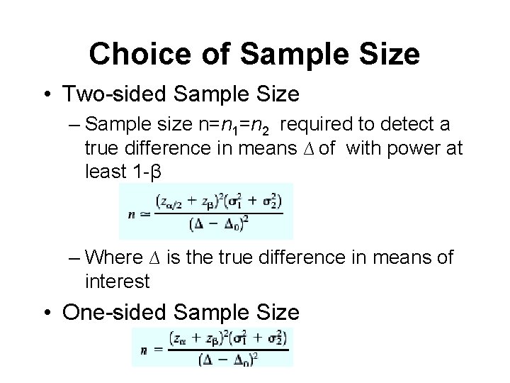
Choice of Sample Size • Two-sided Sample Size – Sample size n=n 1=n 2 required to detect a true difference in means ∆ of with power at least 1 -β – Where ∆ is the true difference in means of interest • One-sided Sample Size

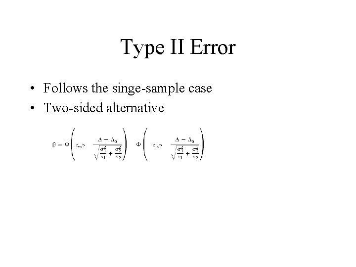
Type II Error • Follows the singe-sample case • Two-sided alternative

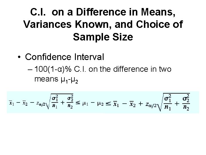
C. I. on a Difference in Means, Variances Known, and Choice of Sample Size • Confidence Interval – 100(1 -α)% C. I. on the difference in two means μ 1 -μ 2

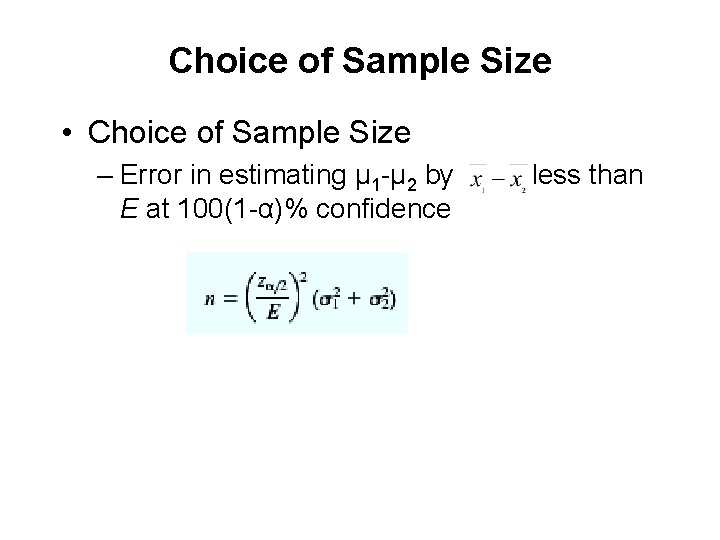
Choice of Sample Size • Choice of Sample Size – Error in estimating μ 1 -μ 2 by E at 100(1 -α)% confidence less than

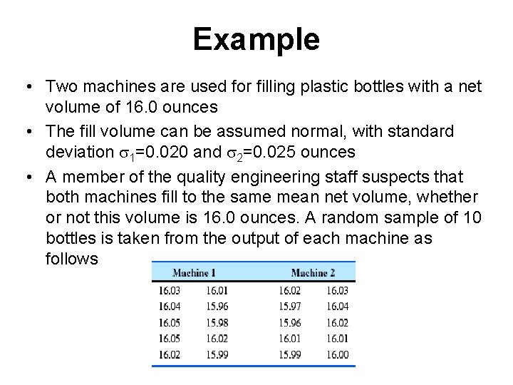
Example • Two machines are used for filling plastic bottles with a net volume of 16. 0 ounces • The fill volume can be assumed normal, with standard deviation 1=0. 020 and 2=0. 025 ounces • A member of the quality engineering staff suspects that both machines fill to the same mean net volume, whether or not this volume is 16. 0 ounces. A random sample of 10 bottles is taken from the output of each machine as follows

Questions 1. 2. 3. 4. 5. Do you think the engineer is correct? Use =0. 05 What is the P-value for this test? What is the power of the test in part (1) for a true difference in means of 0. 04? Find a 95% confidence interval on the difference in means. Provide a practical interpretation of this interval. Assuming equal sample sizes, what sample size should be used to assure that =0. 05 if the true difference in means is 0. 04? Assume that =0. 05

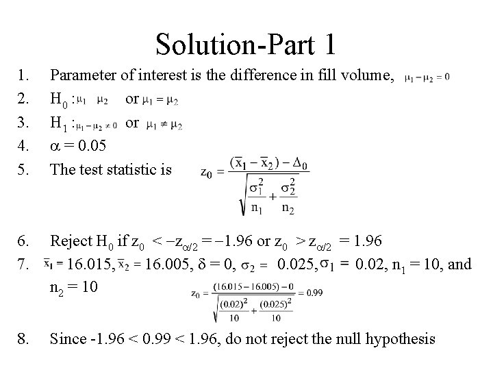
Solution-Part 1 1. 2. 3. 4. 5. Parameter of interest is the difference in fill volume, H 0 : or H 1 : or = 0. 05 The test statistic is 6. 7. Reject H 0 if z 0 < z /2 = 1. 96 or z 0 > z /2 = 1. 96 16. 015, 16. 005, = 0, 0. 025, 0. 02, n 1 = 10, and n 2 = 10 8. Since -1. 96 < 0. 99 < 1. 96, do not reject the null hypothesis

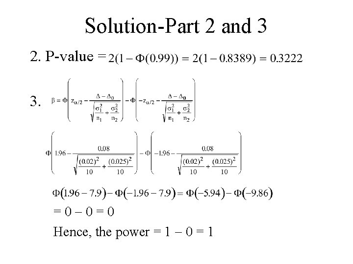
Solution-Part 2 and 3 2. P-value = 3. = 0 0 = 0 Hence, the power = 1 0 = 1

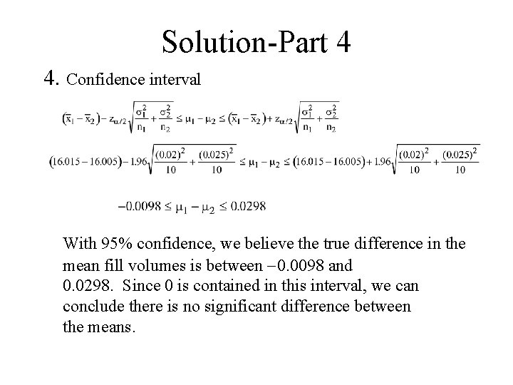
Solution-Part 4 4. Confidence interval With 95% confidence, we believe the true difference in the mean fill volumes is between 0. 0098 and 0. 0298. Since 0 is contained in this interval, we can conclude there is no significant difference between the means.

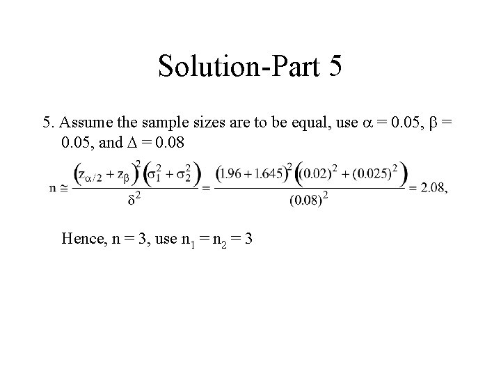
Solution-Part 5 5. Assume the sample sizes are to be equal, use = 0. 05, and = 0. 08 Hence, n = 3, use n 1 = n 2 = 3

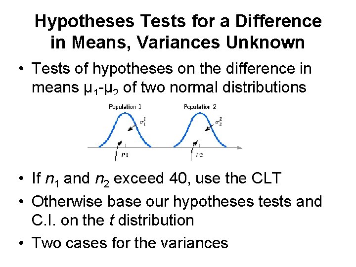
Hypotheses Tests for a Difference in Means, Variances Unknown • Tests of hypotheses on the difference in means μ 1 -μ 2 of two normal distributions • If n 1 and n 2 exceed 40, use the CLT • Otherwise base our hypotheses tests and C. I. on the t distribution • Two cases for the variances

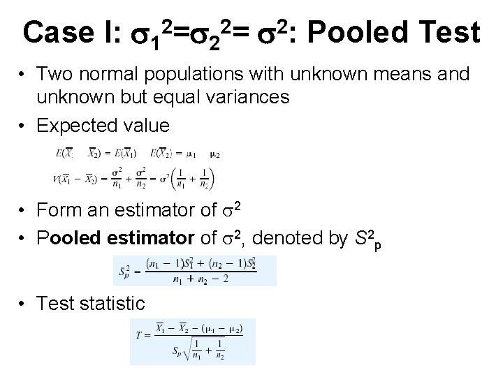
Case I: 12= 2: Pooled Test • Two normal populations with unknown means and unknown but equal variances • Expected value • Form an estimator of 2 • Pooled estimator of 2, denoted by S 2 p • Test statistic

Hypotheses Tests • Test hypothesis – H 0: μ 1 -μ 2 =∆0 – H 1: μ 1 -μ 2 #∆0 • Test statistic • Where Sp is the pooled estimator of

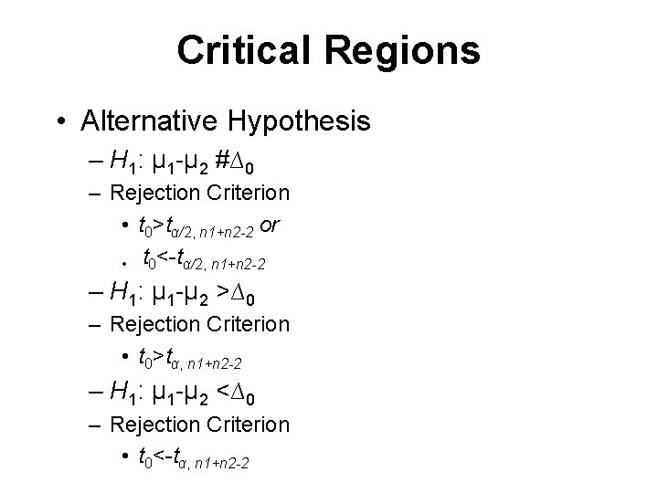
Critical Regions • Alternative Hypothesis – H 1: μ 1 -μ 2 #∆0 – Rejection Criterion • t 0>tα/2, n 1+n 2 -2 or • t 0<-tα/2, n 1+n 2 -2 – H 1: μ 1 -μ 2 >∆0 – Rejection Criterion • t 0>tα, n 1+n 2 -2 – H 1: μ 1 -μ 2 <∆0 – Rejection Criterion • t 0<-tα, n 1+n 2 -2

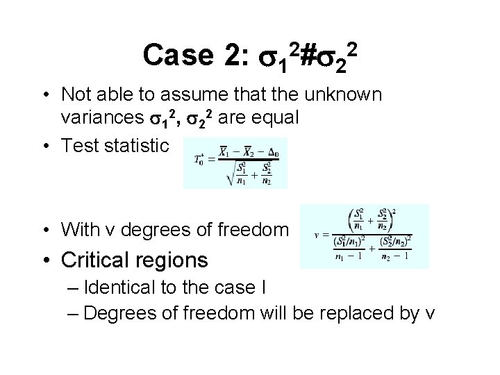
Case 2: 12# 22 • Not able to assume that the unknown variances 12, 22 are equal • Test statistic • With v degrees of freedom • Critical regions – Identical to the case I – Degrees of freedom will be replaced by v

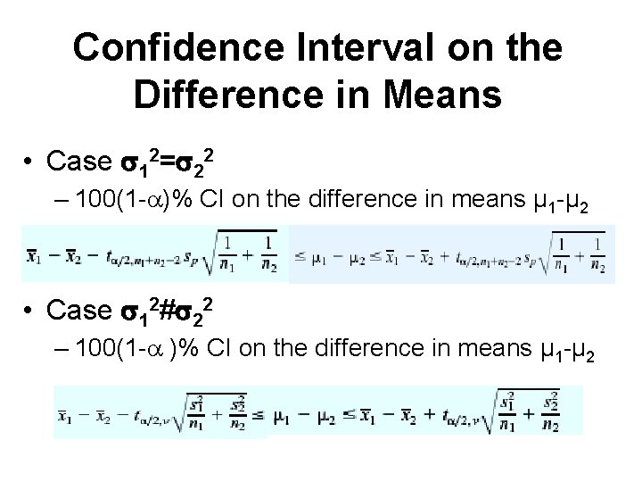
Confidence Interval on the Difference in Means • Case 12= 22 – 100(1 - )% CI on the difference in means μ 1 -μ 2 • Case 12# 22 – 100(1 - )% CI on the difference in means μ 1 -μ 2

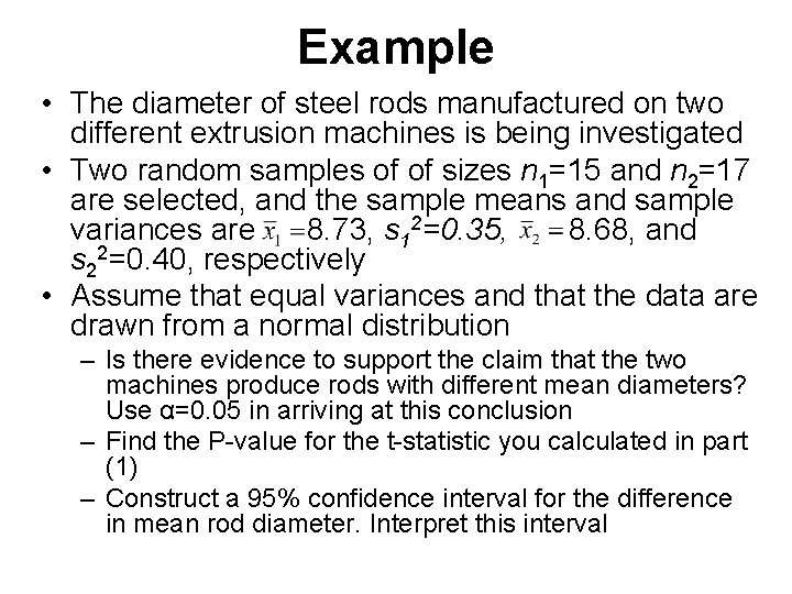
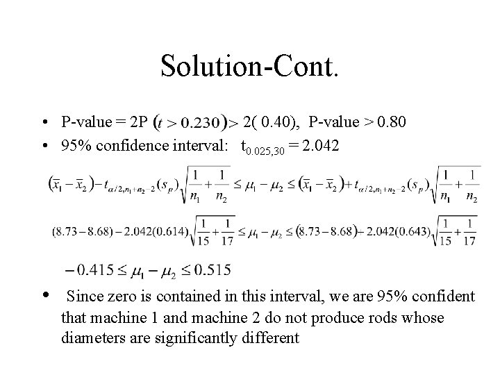
Example • The diameter of steel rods manufactured on two different extrusion machines is being investigated • Two random samples of of sizes n 1=15 and n 2=17 are selected, and the sample means and sample variances are 8. 73, s 12=0. 35, 8. 68, and s 22=0. 40, respectively • Assume that equal variances and that the data are drawn from a normal distribution – Is there evidence to support the claim that the two machines produce rods with different mean diameters? Use α=0. 05 in arriving at this conclusion – Find the P-value for the t-statistic you calculated in part (1) – Construct a 95% confidence interval for the difference in mean rod diameter. Interpret this interval

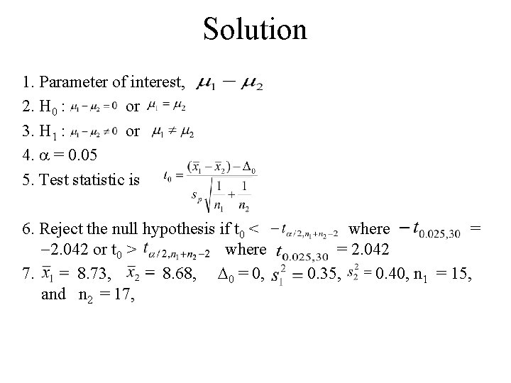
Solution 1. Parameter of interest, 2. H 0 : or 3. H 1 : or 4. = 0. 05 5. Test statistic is 6. Reject the null hypothesis if t 0 < where = 2. 042 or t 0 > where = 2. 042 7. 8. 73, 8. 68, 0 = 0, 0. 35, 0. 40, n 1 = 15, and n 2 = 17,

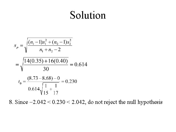
Solution 8. Since 2. 042 < 0. 230 < 2. 042, do not reject the null hypothesis

Solution-Cont. • P-value = 2 P 2( 0. 40), P-value > 0. 80 • 95% confidence interval: t 0. 025, 30 = 2. 042 • Since zero is contained in this interval, we are 95% confident that machine 1 and machine 2 do not produce rods whose diameters are significantly different

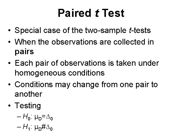
Paired t Test • Special case of the two-sample t-tests • When the observations are collected in pairs • Each pair of observations is taken under homogeneous conditions • Conditions may change from one pair to another • Testing – H 0: μD=∆0 – H 1: μD#∆0

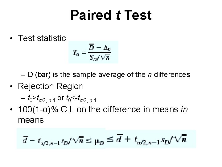
Paired t Test • Test statistic – D (bar) is the sample average of the n differences • Rejection Region – t 0>tα/2, n-1 or t 0<-tα/2, n-1 • 100(1 -α)% C. I. on the difference in means

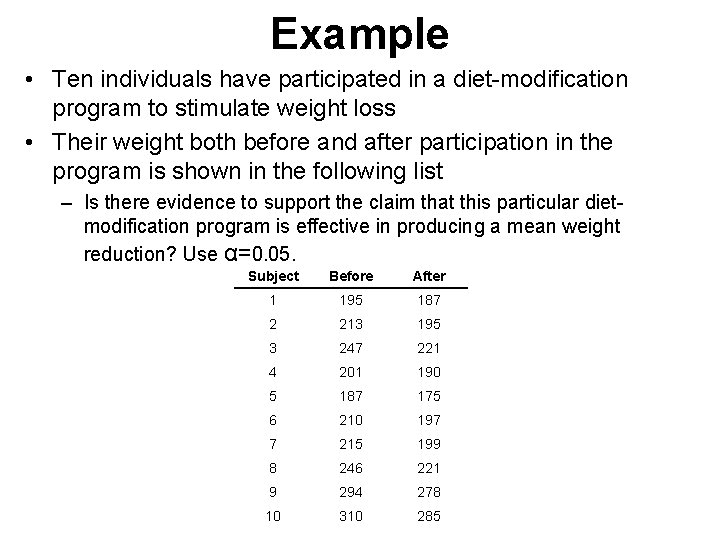
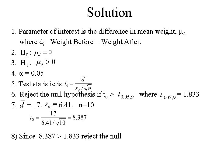
Example • Ten individuals have participated in a diet-modification program to stimulate weight loss • Their weight both before and after participation in the program is shown in the following list – Is there evidence to support the claim that this particular dietmodification program is effective in producing a mean weight reduction? Use α=0. 05. Subject Before After 1 195 187 2 213 195 3 247 221 4 201 190 5 187 175 6 210 197 7 215 199 8 246 221 9 294 278 10 310 285

Solution 1. Parameter of interest is the difference in mean weight, d where di =Weight Before Weight After. 2. H 0 : 3. H 1 : 4. = 0. 05 5. Test statistic is 6. Reject the null hypothesis if t 0 > where = 1. 833 7. 17, 6. 41, n=10 8) Since 8. 387 > 1. 833 reject the null

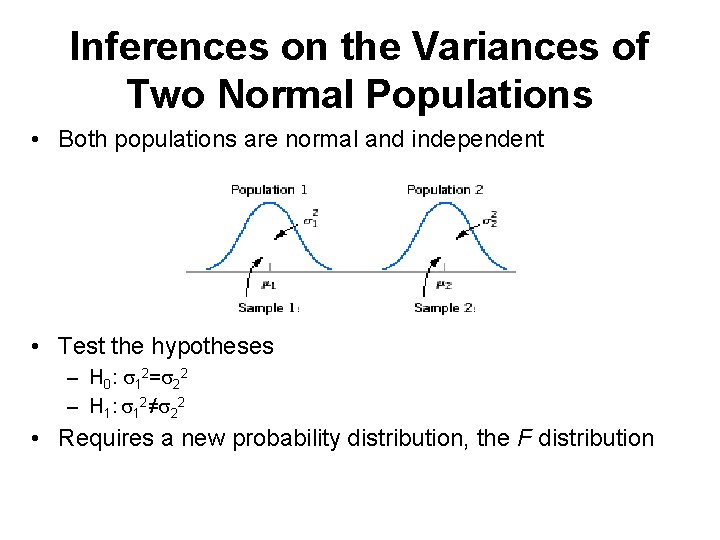
Inferences on the Variances of Two Normal Populations • Both populations are normal and independent • Test the hypotheses – H 0: 12= 22 – H 1: 12≠ 22 • Requires a new probability distribution, the F distribution

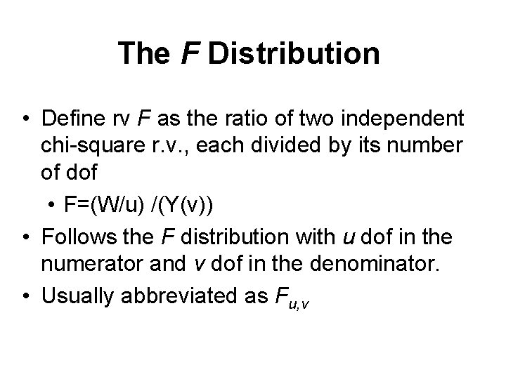
The F Distribution • Define rv F as the ratio of two independent chi-square r. v. , each divided by its number of dof • F=(W/u) /(Y(v)) • Follows the F distribution with u dof in the numerator and v dof in the denominator. • Usually abbreviated as Fu, v

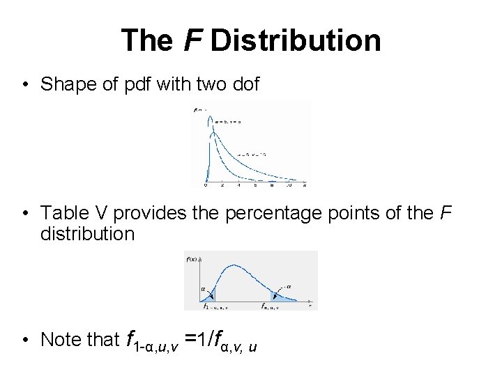
The F Distribution • Shape of pdf with two dof • Table V provides the percentage points of the F distribution • Note that f 1 -α, u, v =1/fα, v, u

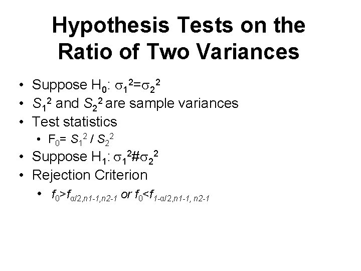
Hypothesis Tests on the Ratio of Two Variances • Suppose H 0: 12= 22 • S 12 and S 22 are sample variances • Test statistics • F 0= S 12 / S 22 • Suppose H 1: 12# 22 • Rejection Criterion • f 0>fα/2, n 1 -1, n 2 -1 or f 0<f 1 -α/2, n 1 -1, n 2 -1

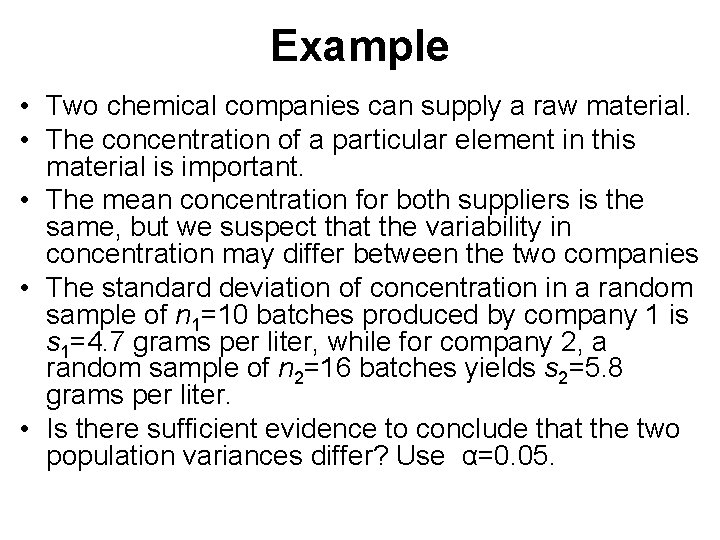
Example • Two chemical companies can supply a raw material. • The concentration of a particular element in this material is important. • The mean concentration for both suppliers is the same, but we suspect that the variability in concentration may differ between the two companies • The standard deviation of concentration in a random sample of n 1=10 batches produced by company 1 is s 1=4. 7 grams per liter, while for company 2, a random sample of n 2=16 batches yields s 2=5. 8 grams per liter. • Is there sufficient evidence to conclude that the two population variances differ? Use α=0. 05.

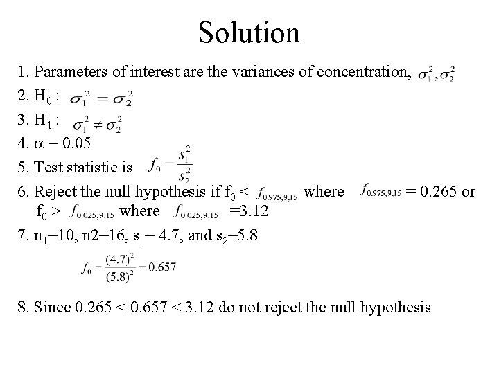
Solution 1. Parameters of interest are the variances of concentration, 2. H 0 : 3. H 1 : 4. = 0. 05 5. Test statistic is 6. Reject the null hypothesis if f 0 < where = 0. 265 or f 0 > where =3. 12 7. n 1=10, n 2=16, s 1= 4. 7, and s 2=5. 8 8. Since 0. 265 < 0. 657 < 3. 12 do not reject the null hypothesis

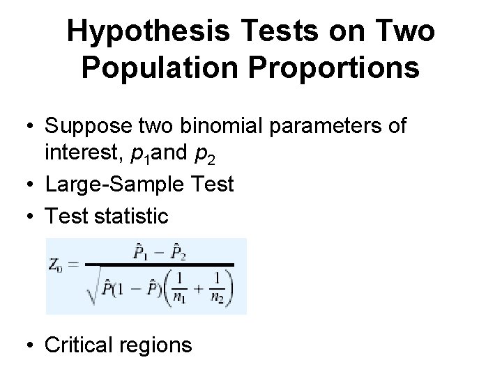
Hypothesis Tests on Two Population Proportions • Suppose two binomial parameters of interest, p 1 and p 2 • Large-Sample Test • Test statistic • Critical regions

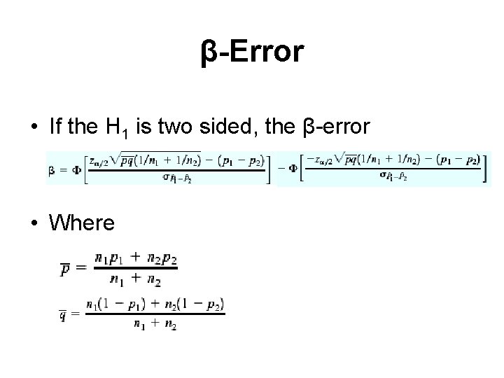
β-Error • If the H 1 is two sided, the β-error • Where

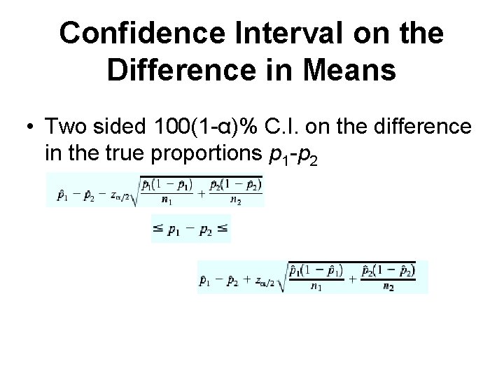
Confidence Interval on the Difference in Means • Two sided 100(1 -α)% C. I. on the difference in the true proportions p 1 -p 2

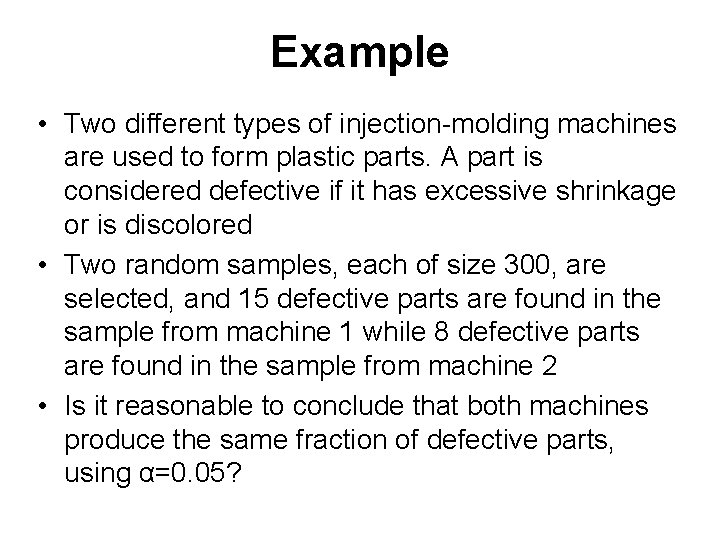
Example • Two different types of injection-molding machines are used to form plastic parts. A part is considered defective if it has excessive shrinkage or is discolored • Two random samples, each of size 300, are selected, and 15 defective parts are found in the sample from machine 1 while 8 defective parts are found in the sample from machine 2 • Is it reasonable to conclude that both machines produce the same fraction of defective parts, using α=0. 05?

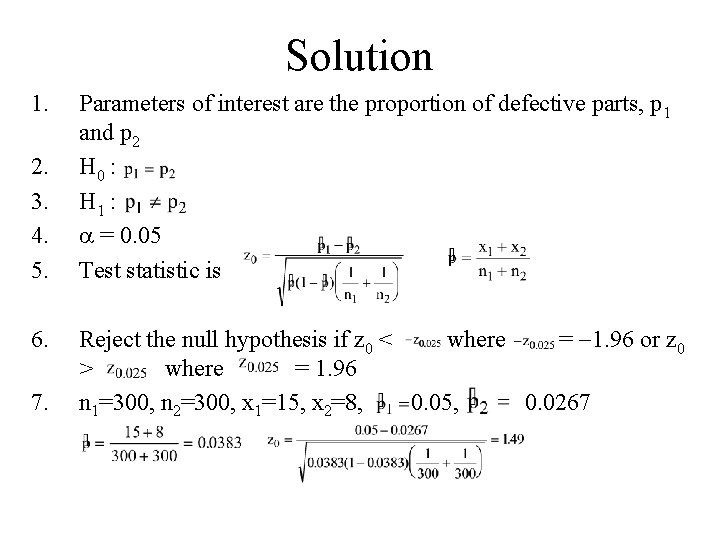
Solution 1. 2. 3. 4. 5. 6. 7. Parameters of interest are the proportion of defective parts, p 1 and p 2 H 0 : H 1 : = 0. 05 Test statistic is Reject the null hypothesis if z 0 < where = 1. 96 or z 0 > where = 1. 96 n 1=300, n 2=300, x 1=15, x 2=8, 0. 05, 0. 0267

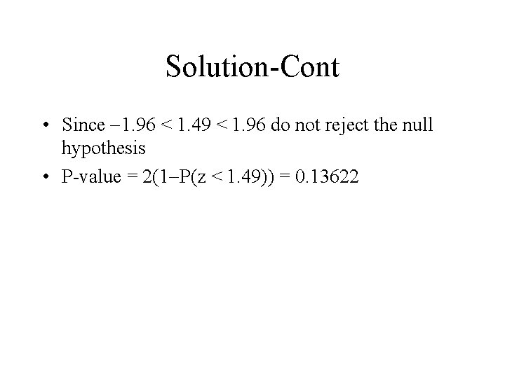
Solution-Cont • Since 1. 96 < 1. 49 < 1. 96 do not reject the null hypothesis • P-value = 2(1 P(z < 1. 49)) = 0. 13622