Chapter 10 Production and Cost Estimation Mc GrawHillIrwin

Chapter 10: Production and Cost Estimation Mc. Graw-Hill/Irwin Copyright © 2011 by the Mc. Graw-Hill Companies, Inc. All rights reserved.

Empirical Production Function • An empirical production function is the mathematical form of the production function to be estimated 10 -2

Empirical Production Function • Long-run production function • A production function in which all inputs are variable • Short-run production function • A production function in which at least one input is fixed 10 -3

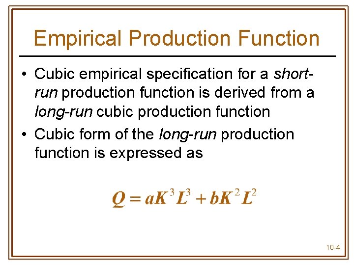
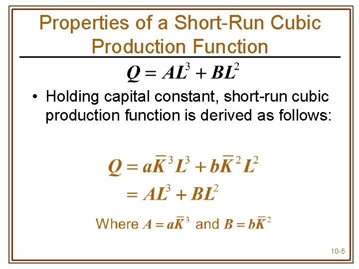
Empirical Production Function • Cubic empirical specification for a shortrun production function is derived from a long-run cubic production function • Cubic form of the long-run production function is expressed as 10 -4

Properties of a Short-Run Cubic Production Function • Holding capital constant, short-run cubic production function is derived as follows: 10 -5

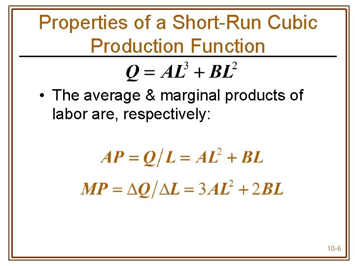
Properties of a Short-Run Cubic Production Function • The average & marginal products of labor are, respectively: 10 -6

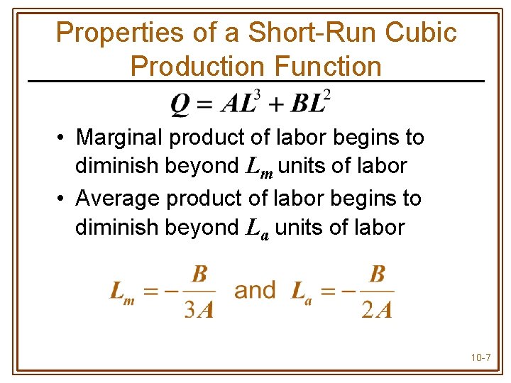
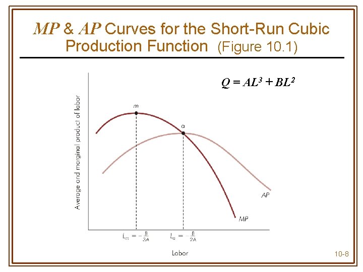
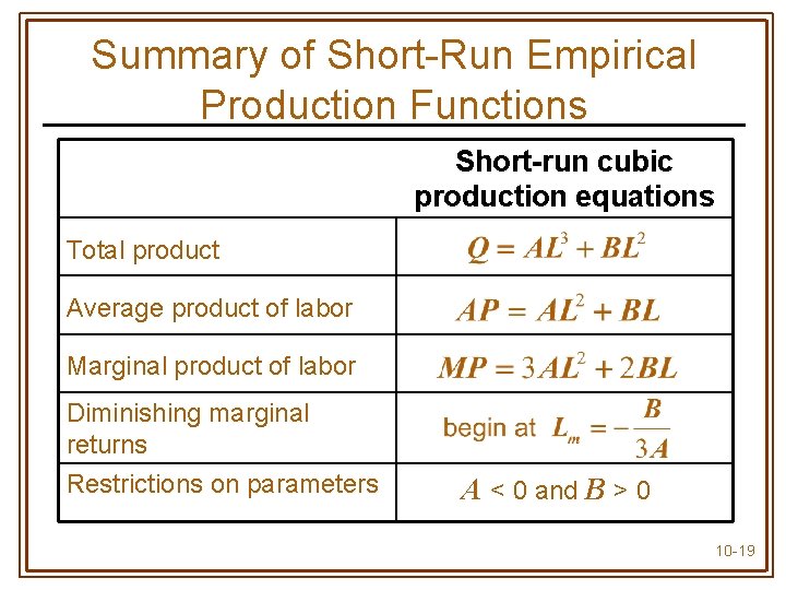
Properties of a Short-Run Cubic Production Function • Marginal product of labor begins to diminish beyond Lm units of labor • Average product of labor begins to diminish beyond La units of labor 10 -7

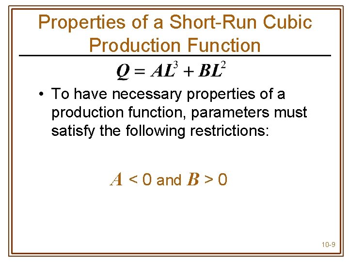
MP & AP Curves for the Short-Run Cubic Production Function (Figure 10. 1) Q = AL 3 + BL 2 10 -8

Properties of a Short-Run Cubic Production Function • To have necessary properties of a production function, parameters must satisfy the following restrictions: A < 0 and B > 0 10 -9

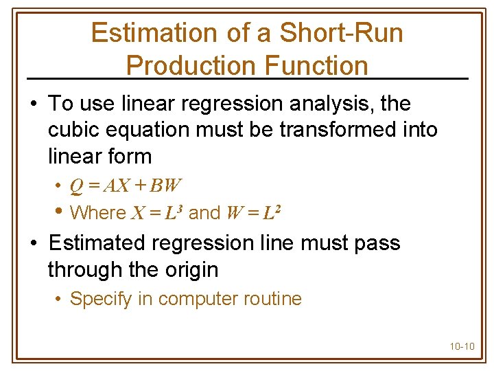
Estimation of a Short-Run Production Function • To use linear regression analysis, the cubic equation must be transformed into linear form • Q = AX + BW • Where X = L 3 and W = L 2 • Estimated regression line must pass through the origin • Specify in computer routine 10 -10

Estimation of a Short-Run Production Function • Estimate using data for which the level of usage of one or more inputs is fixed • Usually time series data are used 10 -11

Estimation of a Short-Run Production Function • Data collection may be complicated by the fact that accounting data do not include firm’s opportunity costs • Capital costs should reflect not only acquisition cost but any foregone rental income, depreciation, & capital gains/losses 10 -12

Estimation of a Short-Run Production Function • Nominal cost data • Data that have not been corrected for the effects of inflation • Must eliminate effects of inflation • Correct for the influence of inflation by dividing nominal cost data by an appropriate price index (or implicit price deflator) 10 -13

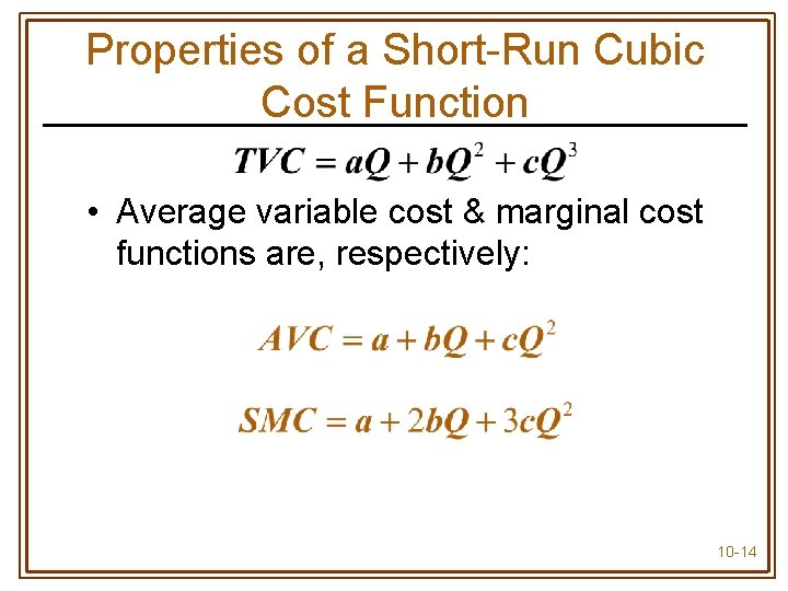
Properties of a Short-Run Cubic Cost Function • Average variable cost & marginal cost functions are, respectively: 10 -14

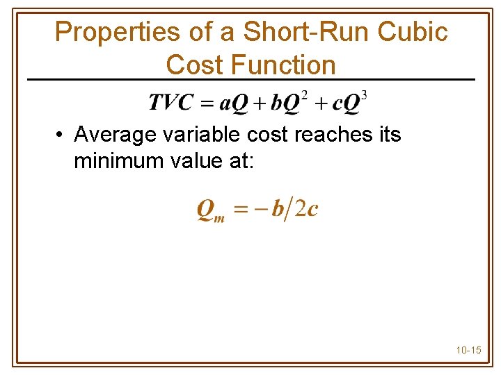
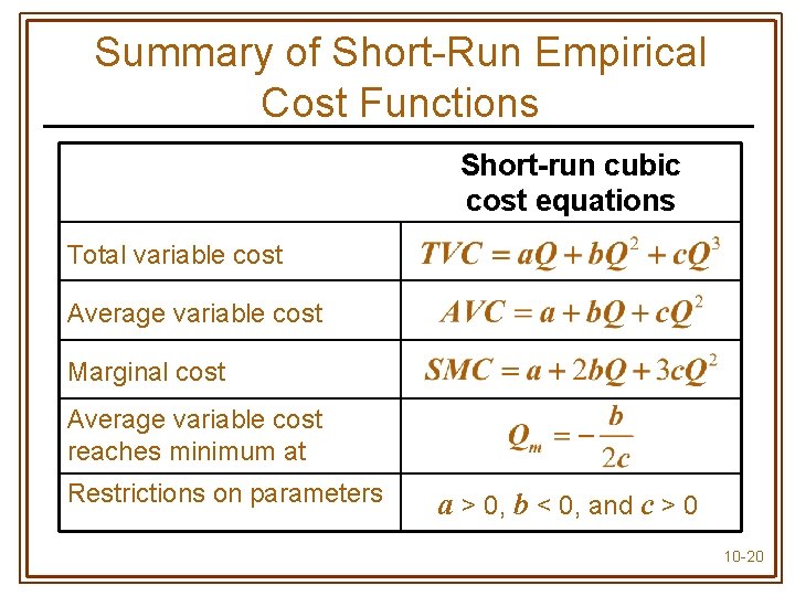
Properties of a Short-Run Cubic Cost Function • Average variable cost reaches its minimum value at: 10 -15

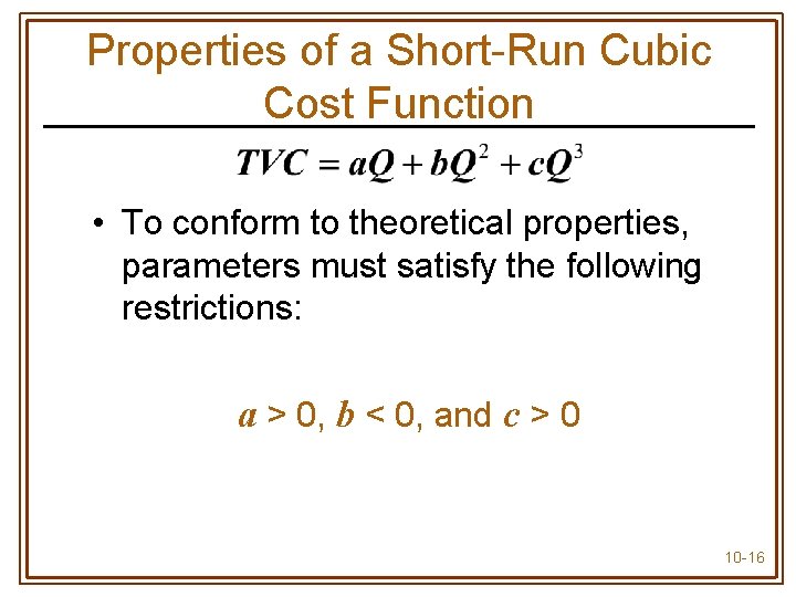
Properties of a Short-Run Cubic Cost Function • To conform to theoretical properties, parameters must satisfy the following restrictions: a > 0, b < 0, and c > 0 10 -16

Properties of a Short-Run Cubic Cost Function • Cubic specification produces S-shaped TVC curve & U-shaped AVC & SMC curves 10 -17

Properties of a Short-Run Cubic Cost Function • All three cost curves employ the same parameters • Only necessary to estimate one of these functions to obtain estimates of all three • In the short-run cubic specification, input prices are assumed constant • Not explicitly included in cost equation 10 -18

Summary of Short-Run Empirical Production Functions Short-run cubic production equations Total product Average product of labor Marginal product of labor Diminishing marginal returns Restrictions on parameters A < 0 and B > 0 10 -19

Summary of Short-Run Empirical Cost Functions Short-run cubic cost equations Total variable cost Average variable cost Marginal cost Average variable cost reaches minimum at Restrictions on parameters a > 0, b < 0, and c > 0 10 -20

Problem Mercantile Metalworks, Inc. manufactures wire carts for grocery stores. The production manager at Mercantile wishes to estimate an empirical production function for the assembly of carts using time-series data for the last 22 days of assembly. L is the daily number of assembly workers employed and Q is the number of carts assembled (completely) for that day. Mercantile pays its assembly workers $160 per day in wages and benefits. 10 -21

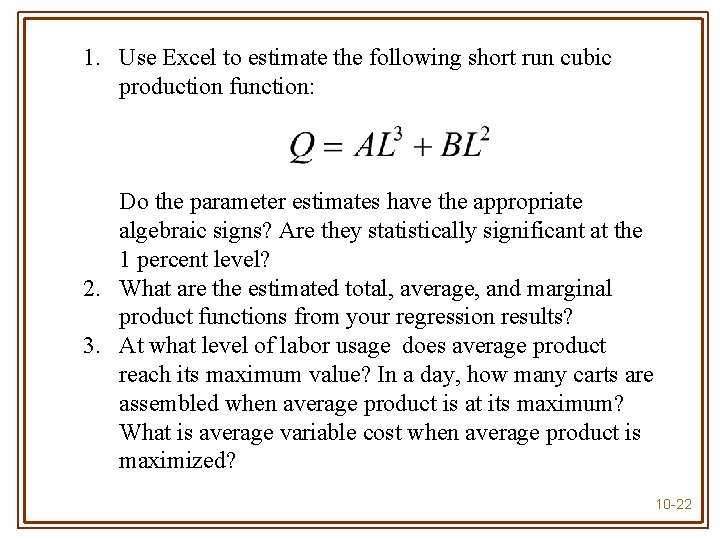
1. Use Excel to estimate the following short run cubic production function: Do the parameter estimates have the appropriate algebraic signs? Are they statistically significant at the 1 percent level? 2. What are the estimated total, average, and marginal product functions from your regression results? 3. At what level of labor usage does average product reach its maximum value? In a day, how many carts are assembled when average product is at its maximum? What is average variable cost when average product is maximized? 10 -22