Chapter 10 Perfect Competition Mc Taggart Findlay Parkin

Chapter 10: Perfect Competition Mc. Taggart, Findlay, Parkin: Microeconomics © 2007 Pearson Education Australia

Objectives After studying this chapter, you will be able to: § Define perfect competition § Explain how firms make their supply decisions and why they sometimes shut down temporarily and lay off workers § Explain how price and output are determined and why firms enter and leave an industry § Predict the effects of a change in demand of a technological advance § Explain why perfect competition is efficient Mc. Taggart, Findlay, Parkin: Microeconomics © 2007 Pearson Education Australia 10 -2

Rivalry in Personal Computers § The personal computer business is a highly competitive business made of such firms as Apple, Dell, Gateway etc competing with hundreds of smaller firms. § How do firms operate when they face the fiercest competition from other firms. What determines their production decisions? Why do firms enter or leave the industry? § These and other questions about competitive markets will be answered in this chapter Mc. Taggart, Findlay, Parkin: Microeconomics © 2007 Pearson Education Australia 10 -3

What is Perfect Competition? § Perfect competition is an industry in which: § Many firms sell identical products to many buyers. § There are no restrictions to entry into the industry. § Existing firms have no advantages over new ones. § Sellers and buyers are well informed about prices. Mc. Taggart, Findlay, Parkin: Microeconomics © 2007 Pearson Education Australia 10 -4

What is Perfect Competition? § How Perfect Competition Arises § Perfect competition arises when two conditions are present: § A firm’s minimum efficient scale is the smallest quantity of output at which long-run average cost reaches its lowest level. § When each firm is perceived to produce a good or service that has no unique characteristics, so consumers don’t care which firm they buy from. Mc. Taggart, Findlay, Parkin: Microeconomics © 2007 Pearson Education Australia 10 -5

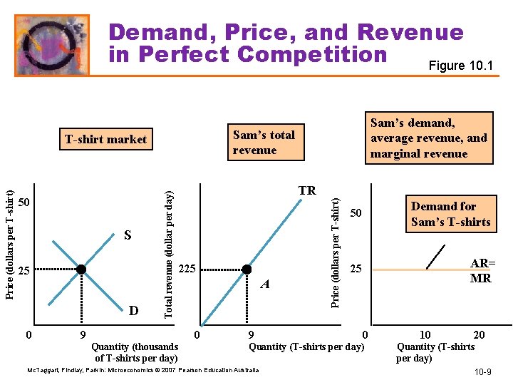
What is Perfect Competition? § Price Takers § In perfect competition, each firm is a price taker. § A price taker is a firm that cannot influence the market price of a good or service. § Each firm produces a tiny fraction of the total output and buyers are well informed about the prices of other firms. § The firm faces a perfectly elastic demand for its output Mc. Taggart, Findlay, Parkin: Microeconomics © 2007 Pearson Education Australia 10 -6

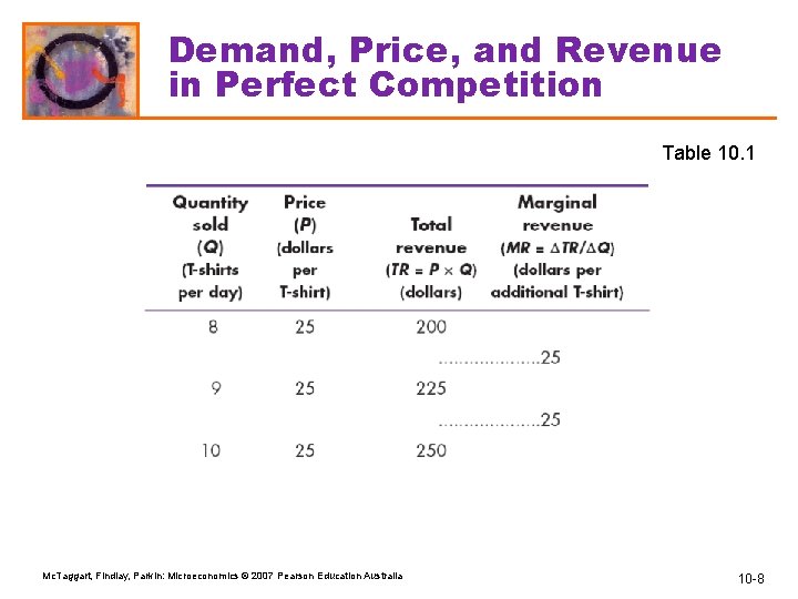
What is Perfect Competition? § Economic Profit and Revenue § The goal of each firm is to maximise economic profit, which equals total revenue minus total cost. § Total cost is the opportunity cost of production, which includes normal profit. § A firm’s total revenue equals price times quantity sold § A firm’s marginal revenue is the change in total revenue that results from a one-unit increase in the quantity sold. Mc. Taggart, Findlay, Parkin: Microeconomics © 2007 Pearson Education Australia 10 -7

Demand, Price, and Revenue in Perfect Competition Table 10. 1 Mc. Taggart, Findlay, Parkin: Microeconomics © 2007 Pearson Education Australia 10 -8

Demand, Price, and Revenue in Perfect Competition Figure 10. 1 Sam’s total revenue 25 D 0 9 TR 225 A 0 Quantity (thousands of T-shirts per day) 9 Price (dollars per T-shirt) S Total revenue (dollar per day) Price (dollars per T-shirt) T-shirt market 50 Sam’s demand, average revenue, and marginal revenue Demand for Sam’s T-shirts 50 AR= MR 25 0 Quantity (T-shirts per day) Mc. Taggart, Findlay, Parkin: Microeconomics © 2007 Pearson Education Australia 10 20 Quantity (T-shirts per day) 10 -9

The Firm’s Decisions in Perfect Competition § A perfectly competitive firm faces two constraints: 1. A market constraint summarised by the market price and the firm’s revenue curves. 2. A technology constraint summarised by the firm’s product curves and cost curves. Mc. Taggart, Findlay, Parkin: Microeconomics © 2007 Pearson Education Australia 10 -10

The Firm’s Decisions in Perfect Competition § Short-Run Decisions § The perfectly competitive firm makes two decisions in the short run: 1. Whether to produce or to temporarily shut down 2. What quantity to produce Mc. Taggart, Findlay, Parkin: Microeconomics © 2007 Pearson Education Australia 10 -11

The Firm’s Decisions in Perfect Competition § Long-Run Decisions § A firm’s long-run decisions are: § Whether to increase or decrease its plant size § Whether to remain in, enter, or leave an industry Mc. Taggart, Findlay, Parkin: Microeconomics © 2007 Pearson Education Australia 10 -12

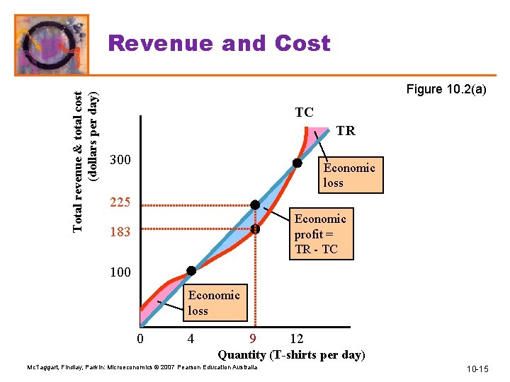
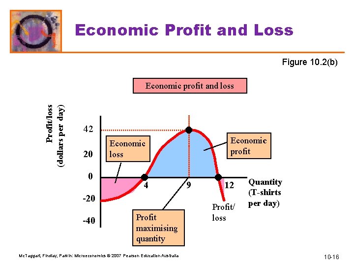
The Firm’s Decisions in Perfect Competition § Profit-Maximising Output § A perfectly competitive firm chooses the output that maximises its economic profit. § One way to find the profit maximising output is to look at the firm’s the total revenue and total cost curves. Mc. Taggart, Findlay, Parkin: Microeconomics © 2007 Pearson Education Australia 10 -13

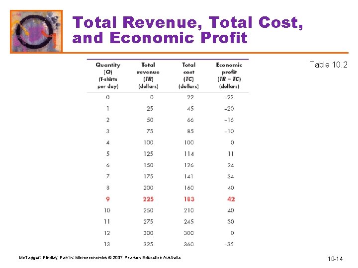
Total Revenue, Total Cost, and Economic Profit Table 10. 2 Mc. Taggart, Findlay, Parkin: Microeconomics © 2007 Pearson Education Australia 10 -14

Total revenue & total cost (dollars per day) Revenue and Cost Figure 10. 2(a) TC TR 300 Economic loss 225 Economic profit = TR - TC 183 100 Economic loss 0 4 9 12 Quantity (T-shirts per day) Mc. Taggart, Findlay, Parkin: Microeconomics © 2007 Pearson Education Australia 10 -15

Economic Profit and Loss Figure 10. 2(b) Profit/loss (dollars per day) Economic profit and loss 42 20 0 4 -20 -40 Economic profit Economic loss Profit maximising quantity Mc. Taggart, Findlay, Parkin: Microeconomics © 2007 Pearson Education Australia 9 12 Profit/ loss Quantity (T-shirts per day) 10 -16

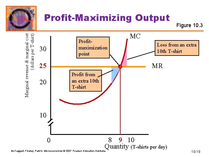
The Firm’s Decisions in Perfect Competition § Marginal Analysis § The firm can use marginal analysis to determine the profitmaximising output. § Profit is maximised by producing the output at which marginal revenue, MR, equals marginal cost, MC. Mc. Taggart, Findlay, Parkin: Microeconomics © 2007 Pearson Education Australia 10 -17

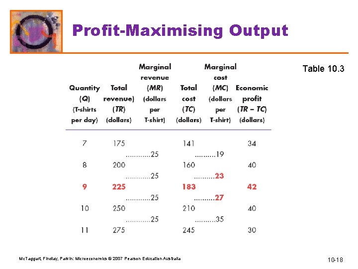
Profit-Maximising Output Table 10. 3 Mc. Taggart, Findlay, Parkin: Microeconomics © 2007 Pearson Education Australia 10 -18

Marginal revenue & marginal cost (dollars per T-shirt) Profit-Maximizing Output Profitmaximization point 30 25 Figure 10. 3 MC Loss from an extra 10 th T-shirt MR Profit from an extra 10 th T-shirt 20 10 0 8 9 10 Quantity (T-shirts per day) Mc. Taggart, Findlay, Parkin: Microeconomics © 2007 Pearson Education Australia 10 -19

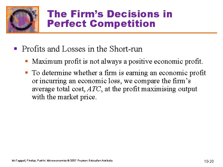
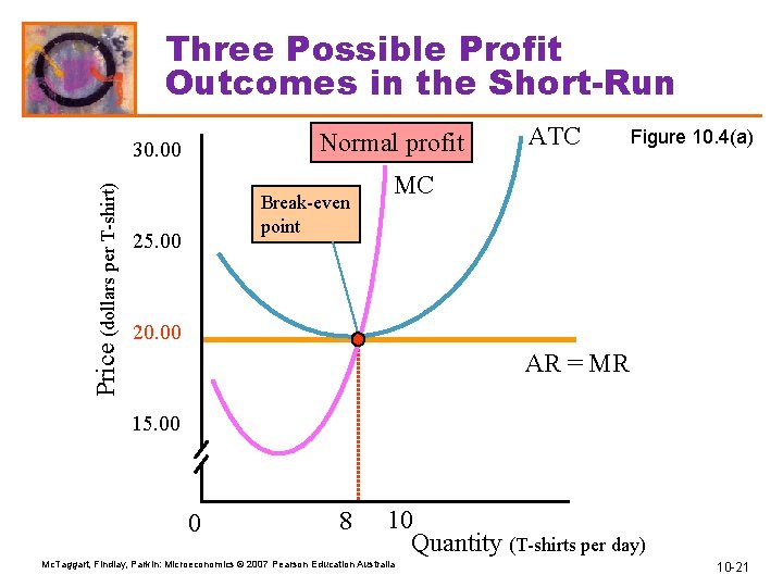
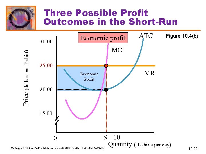
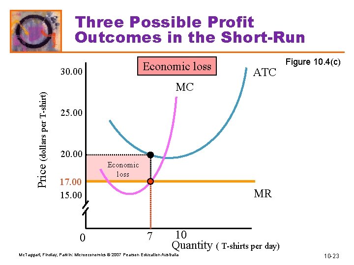
The Firm’s Decisions in Perfect Competition § Profits and Losses in the Short-run § Maximum profit is not always a positive economic profit. § To determine whether a firm is earning an economic profit or incurring an economic loss, we compare the firm’s average total cost, ATC, at the profit maximising output with the market price. Mc. Taggart, Findlay, Parkin: Microeconomics © 2007 Pearson Education Australia 10 -20

Three Possible Profit Outcomes in the Short-Run Normal profit Price (dollars per T-shirt) 30. 00 Break-even point 25. 00 ATC Figure 10. 4(a) MC 20. 00 AR = MR 15. 00 0 8 10 Quantity (T-shirts per day) Mc. Taggart, Findlay, Parkin: Microeconomics © 2007 Pearson Education Australia 10 -21

Three Possible Profit Outcomes in the Short-Run Economic profit Price (dollars per T-shirt) 30. 00 ATC Figure 10. 4(b) MC 25. 00 Economic Profit MR 20. 00 15. 00 0 Mc. Taggart, Findlay, Parkin: Microeconomics © 2007 Pearson Education Australia 9 10 Quantity ( T-shirts per day) 10 -22

Three Possible Profit Outcomes in the Short-Run Economic loss Price (dollars per T-shirt) 30. 00 ATC Figure 10. 4(c) MC 25. 00 20. 00 17. 00 15. 00 0 Economic loss MR 7 10 Quantity ( T-shirts per day) Mc. Taggart, Findlay, Parkin: Microeconomics © 2007 Pearson Education Australia 10 -23

The Firm’s Decisions in Perfect Competition § Temporary Plant Shutdown § If price is less than the minimum average variable cost, the firm shuts down temporarily and incurs a loss equal to total fixed cost. § This loss is the largest that the firm must bear. § If the firm were to produce just 1 unit of output at price below average variable cost, it would incur an additional (and avoidable) loss. Mc. Taggart, Findlay, Parkin: Microeconomics © 2007 Pearson Education Australia 10 -24

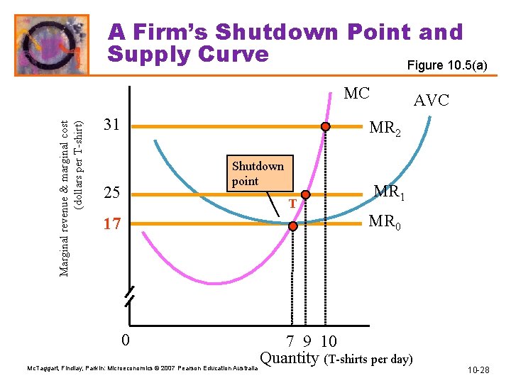
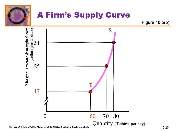
The Firm’s Decisions in Perfect Competition § The Firm’s Short-run Supply Curve § A perfectly competitive firm’s short-run supply curve shows how the firm’s profit-maximising output varies as the market price varies, other things remaining the same. § Because the firm produces the output at which marginal cost equals marginal revenue, and because marginal revenue equals price, the firm’s supply curve is linked to its marginal cost curve. § But there is a price below which the firm produces nothing and shuts down temporarily. Mc. Taggart, Findlay, Parkin: Microeconomics © 2007 Pearson Education Australia 10 -25

The Firm’s Decisions in Perfect Competition § The shutdown point is the output and price at which the firm just covers its total variable cost. § This point is where average variable cost is at its minimum. § It is also the point at which the marginal cost curve crosses the average variable cost curve. § At the shutdown point, the firm is indifferent between producing and shutting down temporarily. § It incurs a loss equal to total fixed cost from either action. Mc. Taggart, Findlay, Parkin: Microeconomics © 2007 Pearson Education Australia 10 -26

The Firm’s Decisions in Perfect Competition § If the price exceeds minimum average variable cost, the firm produces the quantity at which marginal cost equals price. § Price exceeds average variable cost, and the firm covers all its variable cost and at least part of its fixed cost. Mc. Taggart, Findlay, Parkin: Microeconomics © 2007 Pearson Education Australia 10 -27

A Firm’s Shutdown Point and Supply Curve Figure 10. 5(a) Marginal revenue & marginal cost (dollars per T-shirt) MC 31 AVC MR 2 Shutdown point 25 T MR 1 MR 0 17 0 Mc. Taggart, Findlay, Parkin: Microeconomics © 2007 Pearson Education Australia 7 9 10 Quantity (T-shirts per day) 10 -28

A Firm’s Supply Curve Marginal revenue & marginal cost (dollars per T-shirt) Figure 10. 5(b) S 31 25 T 17 0 Mc. Taggart, Findlay, Parkin: Microeconomics © 2007 Pearson Education Australia 60 70 80 Quantity (T-shirts per day) 10 -29

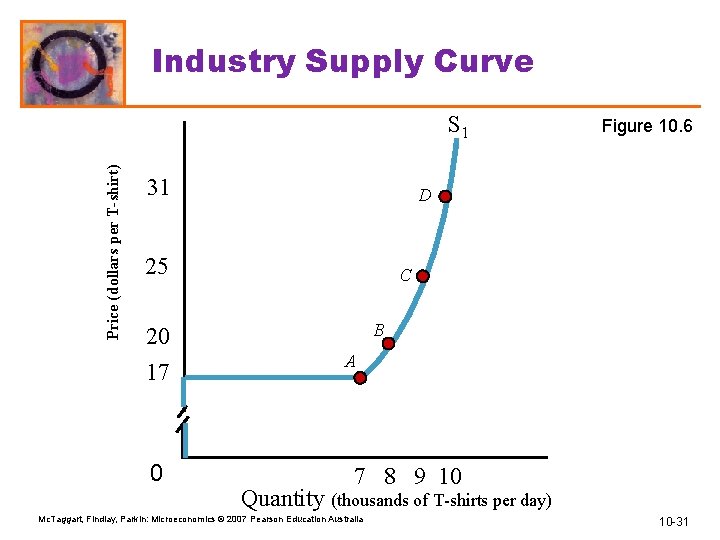
The Firm’s Decisions in Perfect Competition § Short-run Industry Supply Curve § The short-run industry supply curve shows the quantity supplied by the industry at each price when the plant size of each firm and the number of firms remain constant. § The quantity supplied by the industry at any given price is the sum of the quantities supplied by all the firms in the industry at that price. Mc. Taggart, Findlay, Parkin: Microeconomics © 2007 Pearson Education Australia 10 -30

Industry Supply Curve Price (dollars per T-shirt) S 1 31 D 25 C B 20 17 0 Figure 10. 6 A 7 8 9 10 Quantity (thousands of T-shirts per day) Mc. Taggart, Findlay, Parkin: Microeconomics © 2007 Pearson Education Australia 10 -31

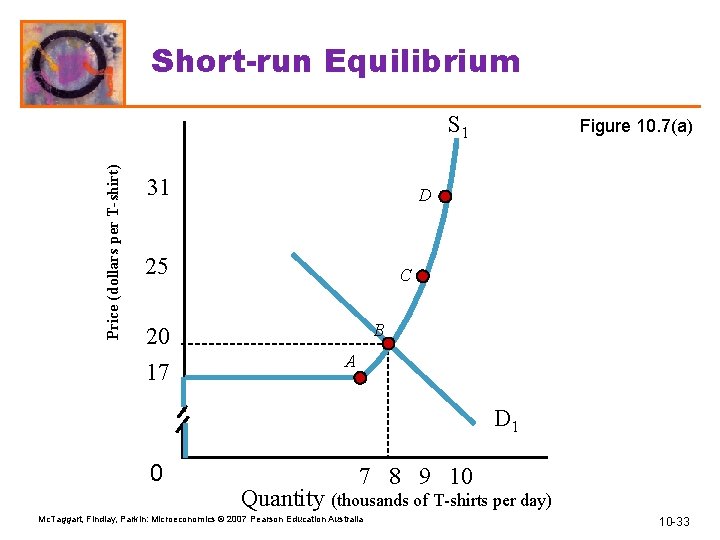
Output, Price, and Profit in Perfect Competition § Short-Run Equilibrium § Short-run industry supply and industry demand determine the market price and output. § A short-run equilibrium occurs at the intersection of the demand supply curves. Mc. Taggart, Findlay, Parkin: Microeconomics © 2007 Pearson Education Australia 10 -32

Short-run Equilibrium Price (dollars per T-shirt) S 1 31 D 25 C B 20 17 Figure 10. 7(a) A D 1 0 7 8 9 10 Quantity (thousands of T-shirts per day) Mc. Taggart, Findlay, Parkin: Microeconomics © 2007 Pearson Education Australia 10 -33

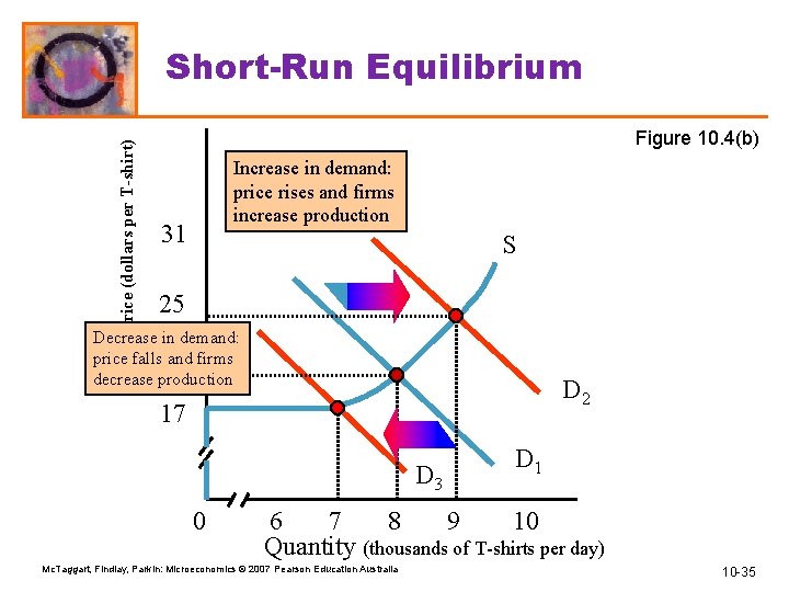
Output, Price, and Profit in Perfect Competition § A Change in Demand § An increase in demand brings a rightward shift of the industry demand curve: the price rises and the quantity increases. § A decrease in demand brings a leftward shift of the industry demand curve: the price falls and the quantity decreases. Mc. Taggart, Findlay, Parkin: Microeconomics © 2007 Pearson Education Australia 10 -34

Price (dollars per T-shirt) Short-Run Equilibrium Figure 10. 4(b) Increase in demand: price rises and firms increase production 31 S 25 Decrease in demand: price falls and firms 20 decrease production D 2 17 D 3 0 D 1 6 7 8 9 10 Quantity (thousands of T-shirts per day) Mc. Taggart, Findlay, Parkin: Microeconomics © 2007 Pearson Education Australia 10 -35

Output, Price, and Profit in Perfect Competition § Long-Run Adjustments § In short-run equilibrium, a firm may earn an economic profit, earn normal profit, or incur an economic loss and which of these states exists determines the further decisions the firm makes in the long run. § In the long run, the firm may: § Enter or exit an industry § Change its plant size Mc. Taggart, Findlay, Parkin: Microeconomics © 2007 Pearson Education Australia 10 -36

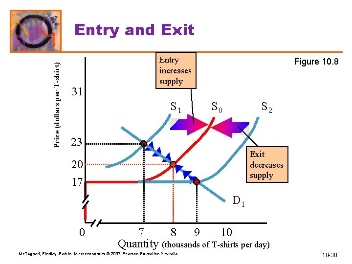
Output, Price, and Profit in Perfect Competition § Entry and Exit § New firms enter an industry in which existing firms earn an economic profit. § Firms exit an industry in which they incur an economic loss. § Entry and exit of new firms shifts the industry supply curve. Mc. Taggart, Findlay, Parkin: Microeconomics © 2007 Pearson Education Australia 10 -37

Price (dollars per T-shirt) Entry and Exit 31 Entry increases supply S 1 Figure 10. 8 S 0 S 2 23 Exit decreases supply 20 17 D 1 0 7 8 9 10 Quantity (thousands of T-shirts per day) Mc. Taggart, Findlay, Parkin: Microeconomics © 2007 Pearson Education Australia 10 -38

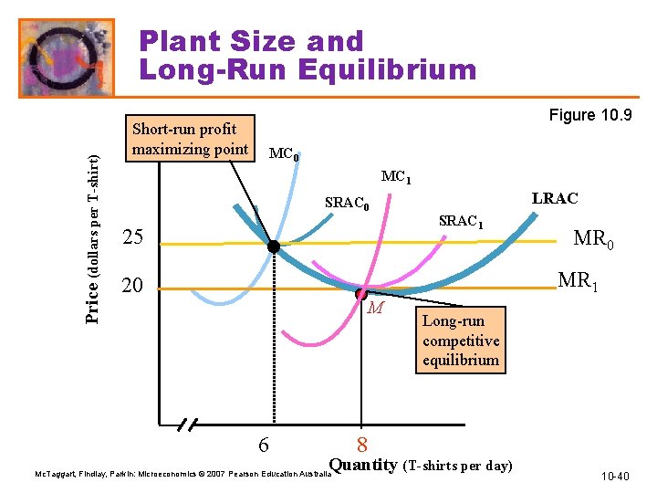
Output, Price, and Profit in Perfect Competition § Changes in Plant Size § Firms change their plant size whenever doing so is profitable. § If average total cost exceeds the minimum long-run average cost, firms change their plant size to lower costs and increase profits. § Figure 10. 9 on the next slide shows the effects of changes in plant size. Mc. Taggart, Findlay, Parkin: Microeconomics © 2007 Pearson Education Australia 10 -39

Price (dollars per T-shirt) Plant Size and Long-Run Equilibrium Figure 10. 9 Short-run profit maximizing point MC 0 MC 1 SRAC 0 25 LRAC SRAC 1 MR 0 MR 1 20 M 6 Long-run competitive equilibrium 8 Quantity (T-shirts per day) Mc. Taggart, Findlay, Parkin: Microeconomics © 2007 Pearson Education Australia 10 -40

Output, Price, and Profit in Perfect Competition § Long-Run Equilibrium § Long-run equilibrium occurs in a competitive industry when: § Economic profit is zero, so firms neither enter nor exit the industry. § Long-run average cost is at its minimum, so firms don’t change their plant size. Mc. Taggart, Findlay, Parkin: Microeconomics © 2007 Pearson Education Australia 10 -41

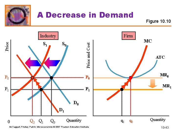
Changing Tastes and Advancing Technology § A Permanent Change in Demand § A decrease in demand shifts the demand curve leftward. The price falls and the quantity decreases. § Economic losses induce exit, which decreases short-run supply and shifts the short-run industry supply curve leftward. Mc. Taggart, Findlay, Parkin: Microeconomics © 2007 Pearson Education Australia 10 -42

A Decrease in Demand Industry S 0 Price and Cost Price S 1 Firm P 0 P 1 Figure 10. 10 MC ATC MR 0 MR 1 D 0 D 1 0 Q 2 Q 1 Q 0 Quantity Mc. Taggart, Findlay, Parkin: Microeconomics © 2007 Pearson Education Australia q 1 q 0 Quantity 10 -43

Changing Tastes and Advancing Technology § Increase in Demand § An increase in demand shifts the demand curve rightward. The price rises and the quantity increases. § Economic profit induces entry, which increases short-run supply and shifts the short-run industry supply curve rightward. § As industry supply increases, the price falls and the market quantity continues to increase. Mc. Taggart, Findlay, Parkin: Microeconomics © 2007 Pearson Education Australia 10 -44

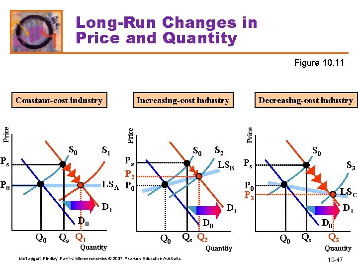
Changing Tastes and Advancing Technology § External Economics and Diseconomies § The change in the long-run equilibrium price following a permanent change in demand depends on external economies and external diseconomies. § External economies are factors beyond the control of an individual firm that lower the firm’s costs as the industry output increases. § External diseconomies are factors beyond the control of a firm that raise the firm’s costs as industry output increases. Mc. Taggart, Findlay, Parkin: Microeconomics © 2007 Pearson Education Australia 10 -45

Changing Tastes and Advancing Technology § A long-run industry supply curve shows how the quantity supplied by an industry varies as the market price varies, after all the possible adjustments have been made, including changes in plant size and changes in the number of firms in the industry Mc. Taggart, Findlay, Parkin: Microeconomics © 2007 Pearson Education Australia 10 -46

Long-Run Changes in Price and Quantity Figure 10. 11 S 0 Ps S 1 LSA P 0 S 2 LSB Ps S 0 Ps P 2 P 0 D 1 D 0 Qs Q 1 Quantity Decreasing-cost industry Price Increasing-cost industry Price Constant-cost industry Q 0 Mc. Taggart, Findlay, Parkin: Microeconomics © 2007 Pearson Education Australia D 0 Qs Q 2 Quantity S 0 S 3 P 0 P 3 LSC D 1 Q 0 Qs D 0 Q 3 Quantity 10 -47

Changing Tastes and Advancing Technology § Technological Change § New technologies are constantly discovered that lower costs. § A new technology enables firms to produce at a lower average cost and lower marginal cost—firms’ cost curves shift downward. § Firms that adopt the new technology earn an economic profit. Mc. Taggart, Findlay, Parkin: Microeconomics © 2007 Pearson Education Australia 10 -48

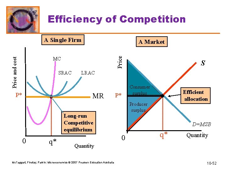
Competition and Efficiency § Efficient Use of Resources § Resource use is efficient when we produce the goods and services that people value most highly § If someone can become better off without anyone else becoming worse off, resources are not being used efficiently. § In other words, resource use is efficient when marginal benefit equals marginal cost. Mc. Taggart, Findlay, Parkin: Microeconomics © 2007 Pearson Education Australia 10 -49

Competition and Efficiency § Choices, Equilibrium, and Efficiency § We can describe an efficient use of resources in terms of the choices of consumers and firms coordinated in market equilibrium. § Consumers allocate their resources to get the most value possible out of them § Consumers get the most value possible out of their resources at all points along their demand curves, which are also their marginal benefit curves. Mc. Taggart, Findlay, Parkin: Microeconomics © 2007 Pearson Education Australia 10 -50

Competition and Efficiency § In competitive equilibrium, the quantity demanded equals the quantity supplied. This means that the consumer’s marginal benefit equals the producer’s marginal cost. § The gains from trade — consumer surplus producer surplus — are maximised. Mc. Taggart, Findlay, Parkin: Microeconomics © 2007 Pearson Education Australia 10 -51

Efficiency of Competition A Single Firm Price A Market Price and cost MC SRAC P* LRAC MR P* q* Consumer surplus Efficient allocation Producer surplus Long-run Competitive equilibrium 0 S D=MSB 0 q* Quantity Mc. Taggart, Findlay, Parkin: Microeconomics © 2007 Pearson Education Australia 10 -52

END CHAPTER 10 Mc. Taggart, Findlay, Parkin: Microeconomics © 2007 Pearson Education Australia 10 -53