Chapter 10 Optimization Designs 10 1 Optimization Designs

Chapter 10 Optimization Designs 10. 1

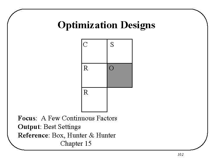
Optimization Designs C S R O R Focus: A Few Continuous Factors Output: Best Settings Reference: Box, Hunter & Hunter Chapter 15 10. 2

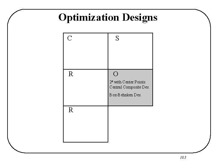
Optimization Designs C S R O 2 k with Center Points Central Composite Des. Box-Behnken Des. R 10. 3

Response Surface Methodology A Strategy of Experimental Design for finding optimum setting for factors. (Box and Wilson, 1951) 10. 4

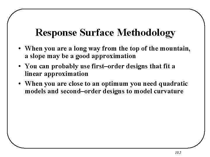
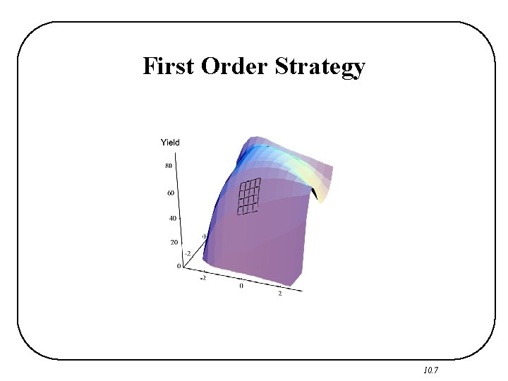
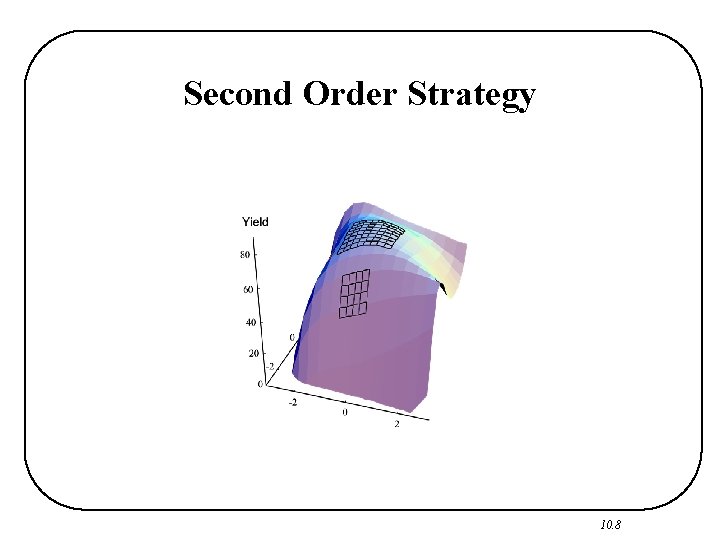
Response Surface Methodology • When you are a long way from the top of the mountain, a slope may be a good approximation • You can probably use first–order designs that fit a linear approximation • When you are close to an optimum you need quadratic models and second–order designs to model curvature 10. 5

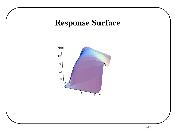
Response Surface 10. 6

First Order Strategy 10. 7

Second Order Strategy 10. 8

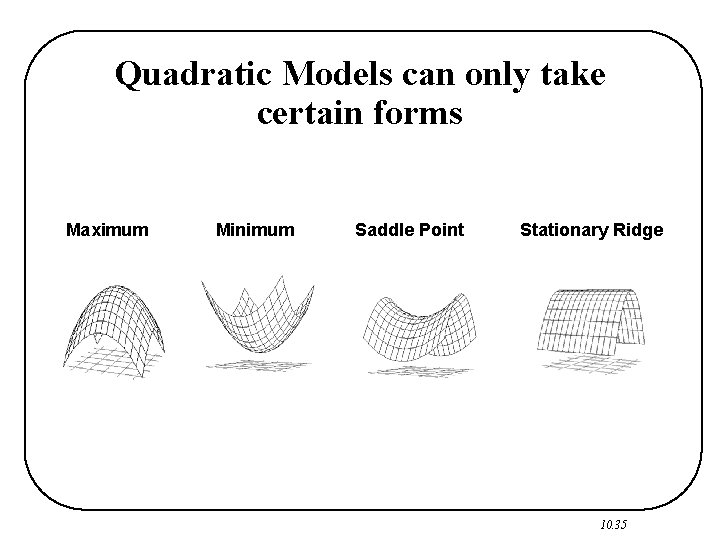
Quadratic Models can only take certain forms Maximum Minimum Saddle Point Stationary Ridge 10. 9

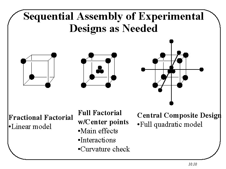
Sequential Assembly of Experimental Designs as Needed Full Factorial Central Composite Design Fractional Factorial w/Center points • Full quadratic model • Linear model • Main effects • Interactions • Curvature check 10. 10

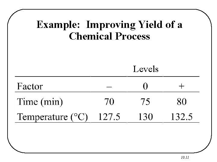
Example: Improving Yield of a Chemical Process Levels 10. 11

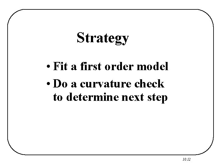
Strategy • Fit a first order model • Do a curvature check to determine next step 10. 12

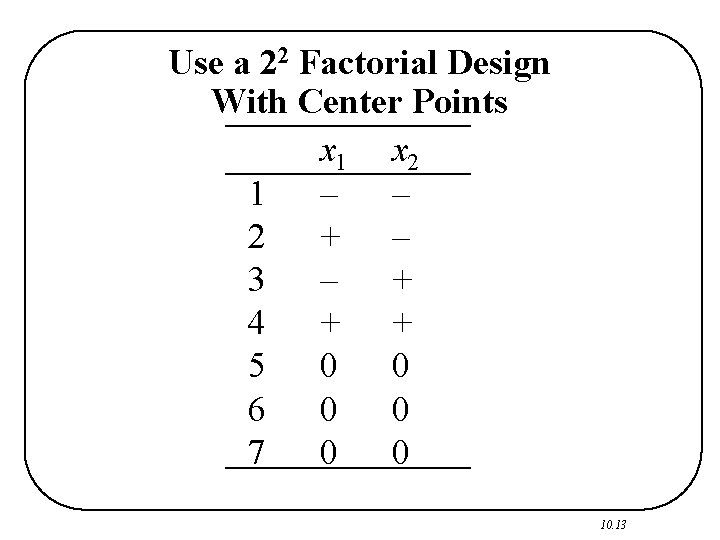
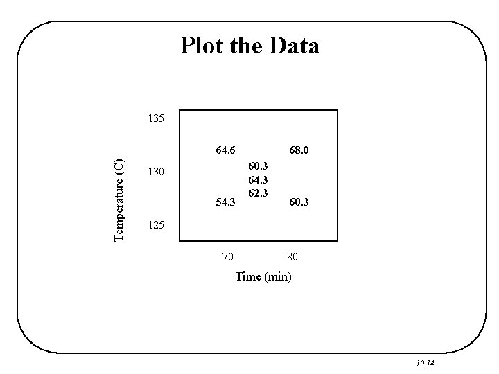
Use a 22 Factorial Design With Center Points x 1 x 2 1 – – 2 + – 3 – + 4 + + 5 0 0 6 0 0 7 0 0 10. 13

Plot the Data 135 Temperature (C) 64. 6 130 54. 3 68. 0 60. 3 64. 3 62. 3 60. 3 125 70 80 Time (min) 10. 14

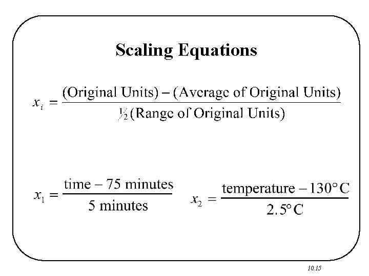
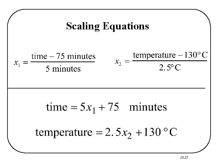
Scaling Equations 10. 15

Results From First Factorial Design 10. 16

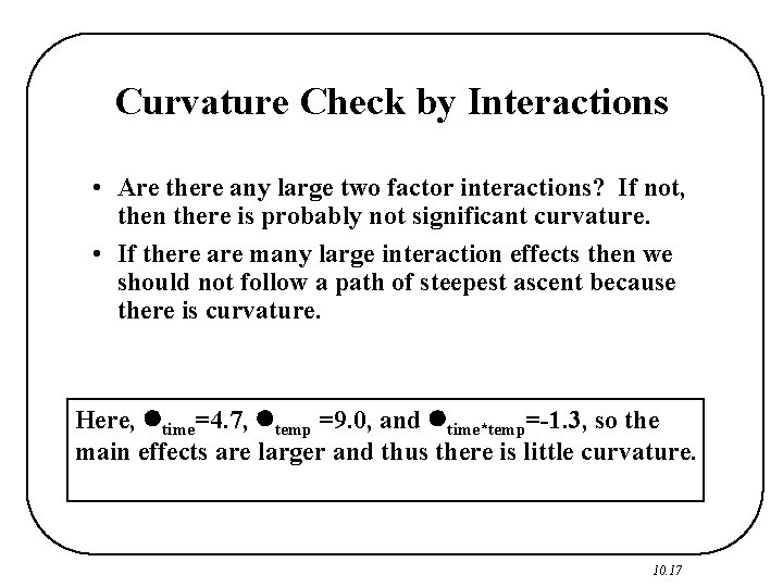
Curvature Check by Interactions • Are there any large two factor interactions? If not, then there is probably not significant curvature. • If there are many large interaction effects then we should not follow a path of steepest ascent because there is curvature. Here, time=4. 7, temp =9. 0, and time*temp=-1. 3, so the main effects are larger and thus there is little curvature. 10. 17

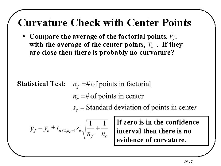
Curvature Check with Center Points • Compare the average of the factorial points, , with the average of the center points, . If they are close then there is probably no curvature? Statistical Test: If zero is in the confidence interval then there is no evidence of curvature. 10. 18

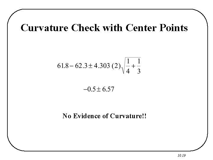
Curvature Check with Center Points No Evidence of Curvature!! 10. 19

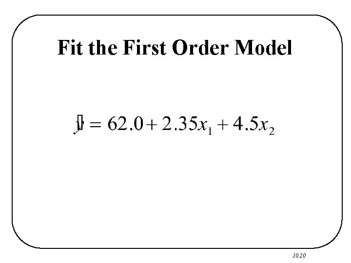
Fit the First Order Model 10. 20

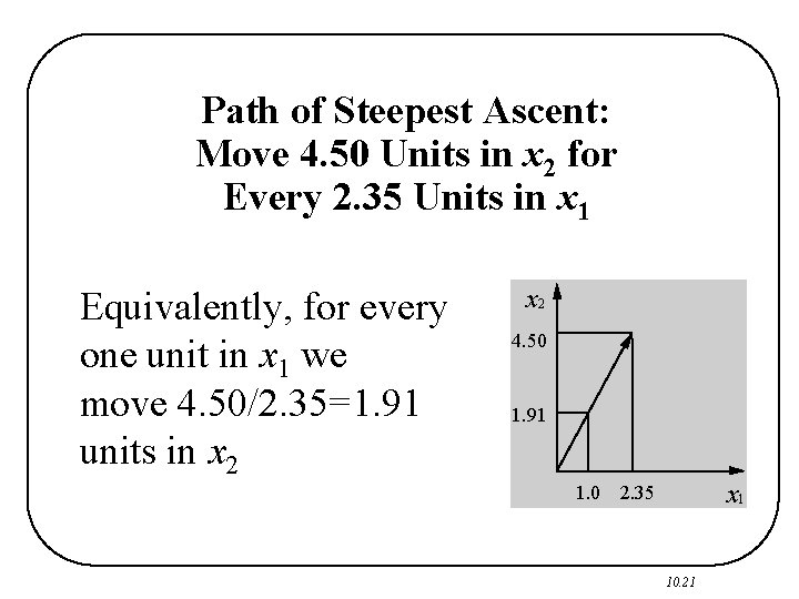
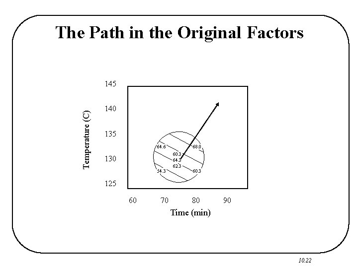
Path of Steepest Ascent: Move 4. 50 Units in x 2 for Every 2. 35 Units in x 1 Equivalently, for every one unit in x 1 we move 4. 50/2. 35=1. 91 units in x 2 4. 50 1. 91 x 1 1. 0 2. 35 10. 21

The Path in the Original Factors Temperature (C) 145 140 135 64. 6 130 54. 3 68. 0 60. 3 64. 3 62. 3 60. 3 125 60 70 80 90 Time (min) 10. 22

Scaling Equations 10. 23

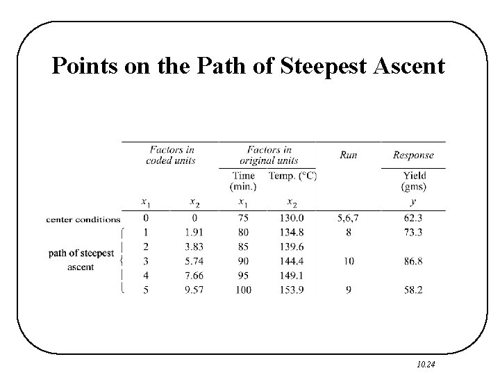
Points on the Path of Steepest Ascent 10. 24

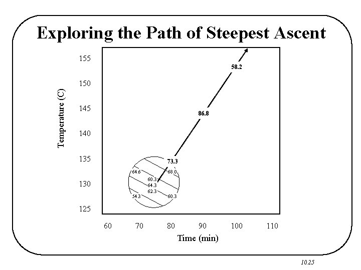
Exploring the Path of Steepest Ascent 155 58. 2 Temperature (C) 150 145 86. 8 140 135 73. 3 64. 6 130 54. 3 68. 0 60. 3 64. 3 62. 3 60. 3 125 60 70 80 90 100 110 Time (min) 10. 25

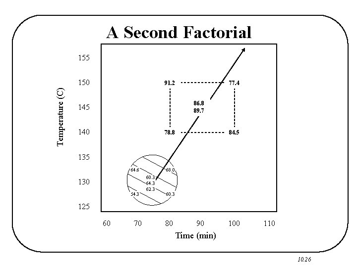
A Second Factorial 155 Temperature (C) 150 91. 2 77. 4 86. 8 89. 7 145 140 78. 8 84. 5 135 64. 6 130 54. 3 68. 0 60. 3 64. 3 62. 3 60. 3 125 60 70 80 90 100 110 Time (min) 10. 26

Results of Second Factorial Design 10. 27

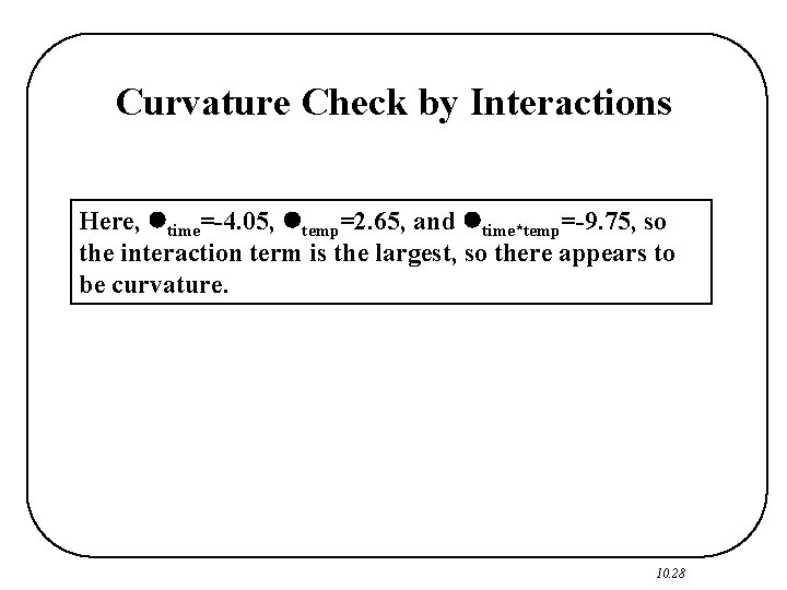
Curvature Check by Interactions Here, time=-4. 05, temp=2. 65, and time*temp=-9. 75, so the interaction term is the largest, so there appears to be curvature. 10. 28

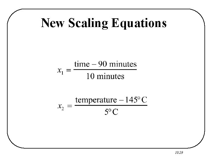
New Scaling Equations 10. 29

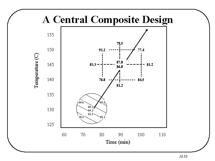
A Central Composite Design 155 79. 5 Temperature (C) 150 91. 2 145 87. 0 86. 0 83. 3 140 77. 4 78. 8 81. 2 84. 5 81. 2 135 64. 6 130 54. 3 68. 0 60. 3 64. 3 62. 3 60. 3 125 60 70 80 90 100 110 Time (min) 10. 30

The Central Composite Design and Results 10. 31

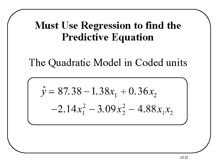
Must Use Regression to find the Predictive Equation The Quadratic Model in Coded units 10. 32

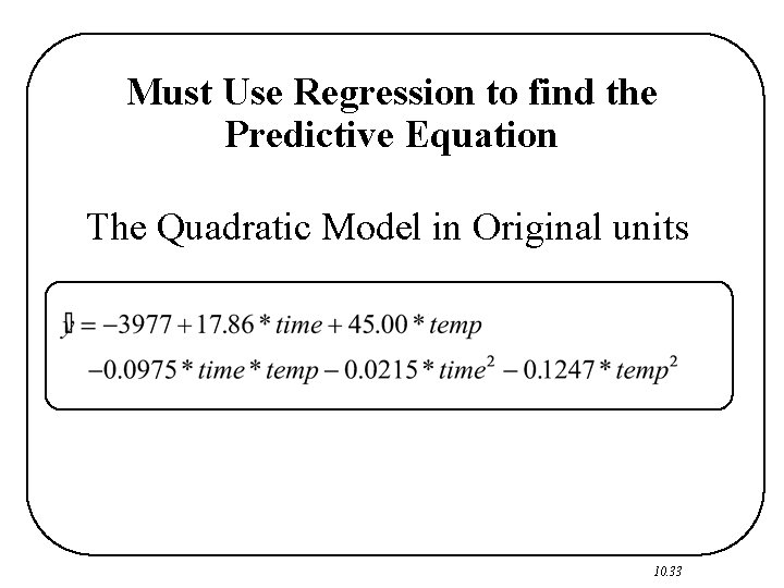
Must Use Regression to find the Predictive Equation The Quadratic Model in Original units 10. 33

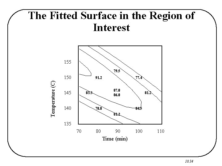
The Fitted Surface in the Region of Interest 155 79. 5 Temperature (C) 150 91. 2 145 87. 0 86. 0 83. 3 140 77. 4 78. 8 81. 2 84. 5 81. 2 135 70 80 90 100 110 Time (min) 10. 34

Quadratic Models can only take certain forms Maximum Minimum Saddle Point Stationary Ridge 10. 35

Canonical Analysis Enables us to analyze systems of maxima and minima in many dimensions and, in particular to identify complicated ridge systems, where direct geometric representation is not possible. 10. 36

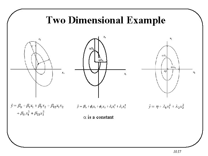
Two Dimensional Example x 2 x 1 is a constant 10. 37

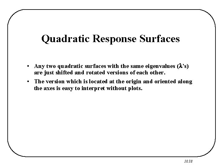
Quadratic Response Surfaces • Any two quadratic surfaces with the same eigenvalues ( ’s) are just shifted and rotated versions of each other. • The version which is located at the origin and oriented along the axes is easy to interpret without plots. 10. 38

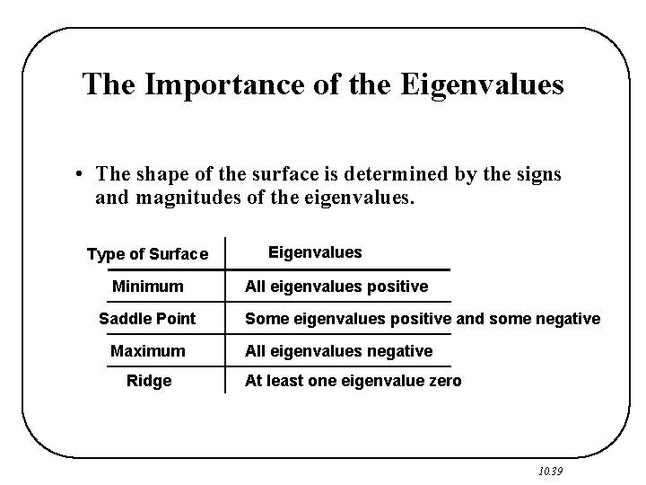
The Importance of the Eigenvalues • The shape of the surface is determined by the signs and magnitudes of the eigenvalues. Type of Surface Minimum Saddle Point Maximum Ridge Eigenvalues All eigenvalues positive Some eigenvalues positive and some negative All eigenvalues negative At least one eigenvalue zero 10. 39

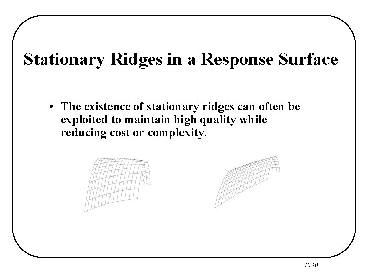
Stationary Ridges in a Response Surface • The existence of stationary ridges can often be exploited to maintain high quality while reducing cost or complexity. 10. 40

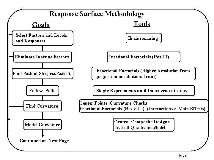
Response Surface Methodology Tools Goals Select Factors and Levels and Responses Eliminate Inactive Factors Find Path of Steepest Ascent Brainstorming Fractional Factorials (Res III) Fractional Factorials (Higher Resolution from projection or additional runs) Follow Path Single Experiments until Improvement stops Find Curvature Center Points (Curvature Check) Fractional Factorials (Res > III) (Interactions > Main Effects) Model Curvature Central Composite Designs Fit Full Quadratic Model Continued on Next Page 10. 41

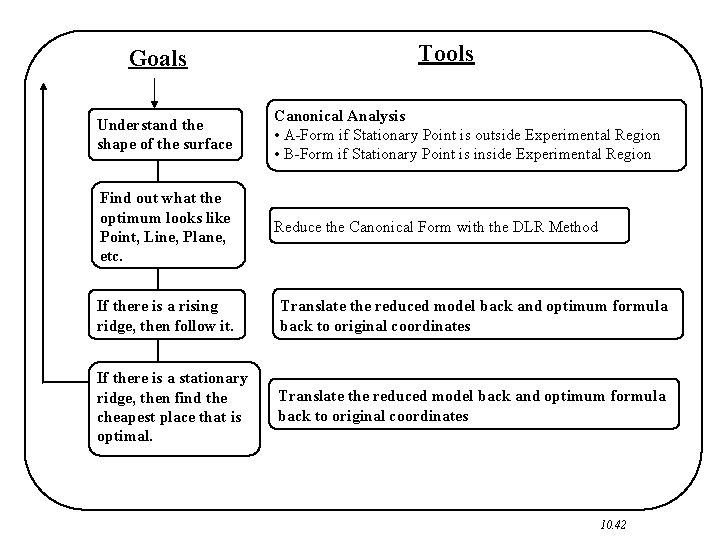
Goals Tools Understand the shape of the surface Canonical Analysis • A-Form if Stationary Point is outside Experimental Region • B-Form if Stationary Point is inside Experimental Region Find out what the optimum looks like Point, Line, Plane, etc. Reduce the Canonical Form with the DLR Method If there is a rising ridge, then follow it. Translate the reduced model back and optimum formula back to original coordinates If there is a stationary ridge, then find the cheapest place that is optimal. Translate the reduced model back and optimum formula back to original coordinates 10. 42