Chapter 10 Money Interest and Income Introduction Money

Chapter 10 Money, Interest, and Income

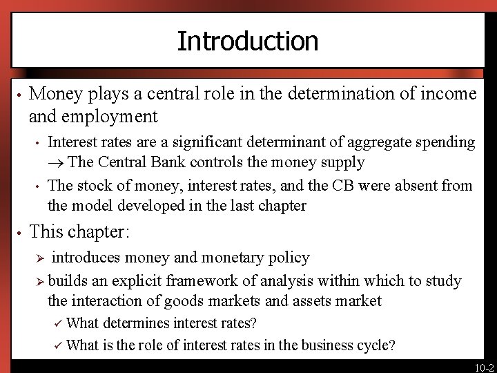
Introduction • Money plays a central role in the determination of income and employment • • • Interest rates are a significant determinant of aggregate spending The Central Bank controls the money supply The stock of money, interest rates, and the CB were absent from the model developed in the last chapter This chapter: introduces money and monetary policy Ø builds an explicit framework of analysis within which to study the interaction of goods markets and assets market Ø What determines interest rates? ü What is the role of interest rates in the business cycle? ü 10 -2

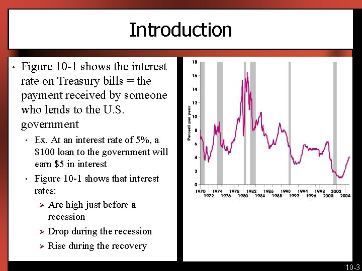
Introduction • Figure 10 -1 shows the interest rate on Treasury bills = the payment received by someone who lends to the U. S. government • • [Insert Figure 10 -1 here] Ex. At an interest rate of 5%, a $100 loan to the government will earn $5 in interest Figure 10 -1 shows that interest rates: Ø Are high just before a recession Ø Drop during the recession Ø Rise during the recovery 10 -3

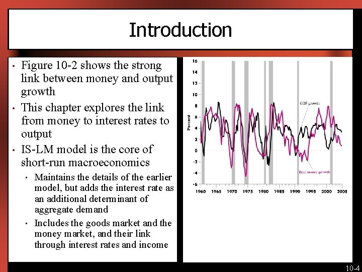
Introduction • • • Figure 10 -2 shows the strong link between money and output growth This chapter explores the link from money to interest rates to output IS-LM model is the core of short-run macroeconomics • • [Insert Figure 10 -2 here] Maintains the details of the earlier model, but adds the interest rate as an additional determinant of aggregate demand Includes the goods market and the money market, and their link through interest rates and income 10 -4

Introduction [Insert Figure 10 -3 here] 10 -5

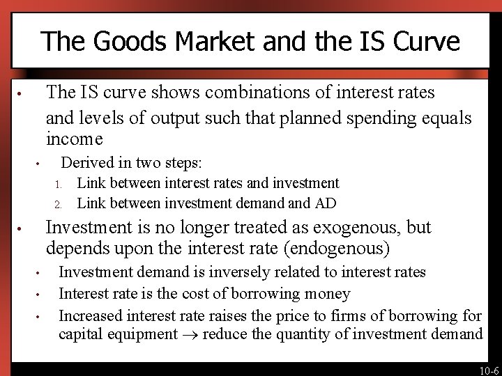
The Goods Market and the IS Curve The IS curve shows combinations of interest rates and levels of output such that planned spending equals income • • Derived in two steps: 1. 2. Link between interest rates and investment Link between investment demand AD Investment is no longer treated as exogenous, but depends upon the interest rate (endogenous) • • Investment demand is inversely related to interest rates Interest rate is the cost of borrowing money Increased interest rate raises the price to firms of borrowing for capital equipment reduce the quantity of investment demand 10 -6

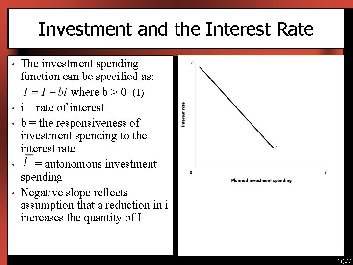
Investment and the Interest Rate • • • The investment spending function can be specified as: where b > 0 (1) i = rate of interest b = the responsiveness of investment spending to the interest rate = autonomous investment spending Negative slope reflects assumption that a reduction in i increases the quantity of I [Insert Figure 10 -4 here] 10 -7

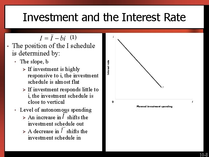
Investment and the Interest Rate (1) • The position of the I schedule is determined by: • • [Insert Figure 10 -4 here] The slope, b Ø If investment is highly responsive to i, the investment schedule is almost flat Ø If investment responds little to i, the investment schedule is close to vertical Level of autonomous spending Ø An increase in shifts the investment schedule out Ø A decrease in shifts the investment schedule in 10 -8

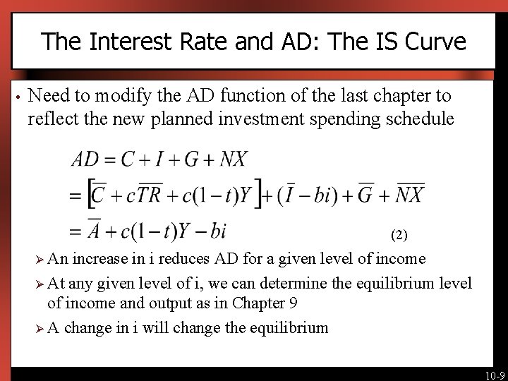
The Interest Rate and AD: The IS Curve • Need to modify the AD function of the last chapter to reflect the new planned investment spending schedule (2) Ø An increase in i reduces AD for a given level of income Ø At any given level of i, we can determine the equilibrium level of income and output as in Chapter 9 Ø A change in i will change the equilibrium 10 -9

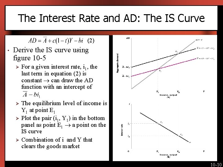
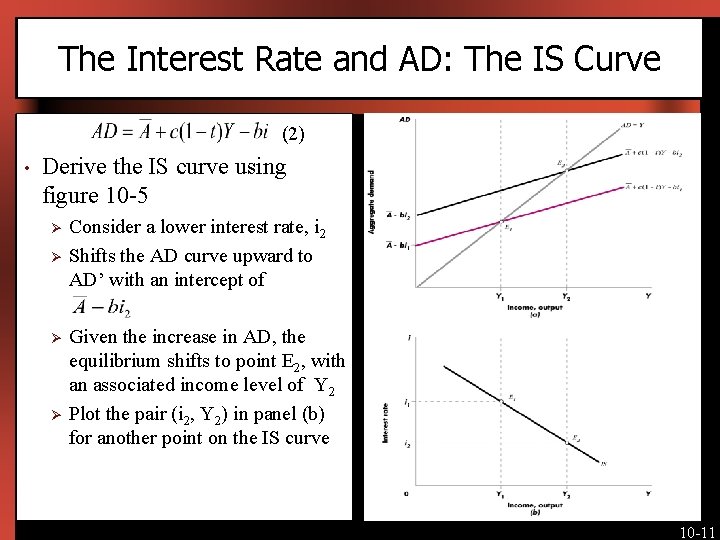
The Interest Rate and AD: The IS Curve (2) • [Insert Figure 10 -5 here] Derive the IS curve using figure 10 -5 Ø For a given interest rate, i 1, the last term in equation (2) is constant can draw the AD function with an intercept of Ø The equilibrium level of income is Y 1 at point E 1 Plot the pair (i 1, Y 1) in the bottom panel as point E 1 a point on the IS curve Combination of i and Y that clears the goods market Ø Ø 10 -10

The Interest Rate and AD: The IS Curve (2) • [Insert Figure 10 -5 here again] Derive the IS curve using figure 10 -5 Ø Ø Consider a lower interest rate, i 2 Shifts the AD curve upward to AD’ with an intercept of Given the increase in AD, the equilibrium shifts to point E 2, with an associated income level of Y 2 Plot the pair (i 2, Y 2) in panel (b) for another point on the IS curve 10 -11

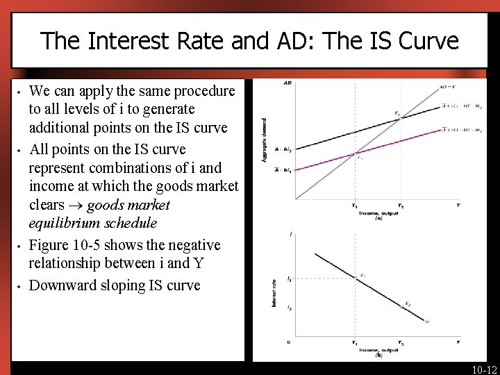
The Interest Rate and AD: The IS Curve • • We can apply the same procedure to all levels of i to generate additional points on the IS curve All points on the IS curve represent combinations of i and income at which the goods market clears goods market equilibrium schedule Figure 10 -5 shows the negative relationship between i and Y Downward sloping IS curve [Insert Figure 10 -5 here again] 10 -12

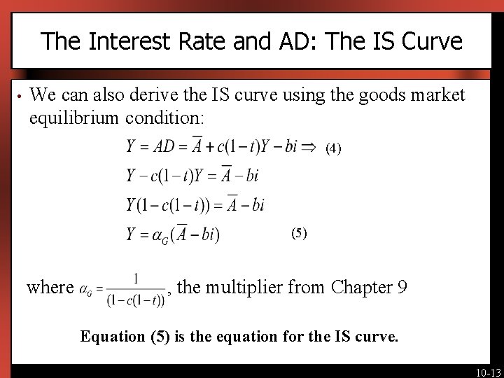
The Interest Rate and AD: The IS Curve • We can also derive the IS curve using the goods market equilibrium condition: (4) (5) where , the multiplier from Chapter 9 Equation (5) is the equation for the IS curve. 10 -13

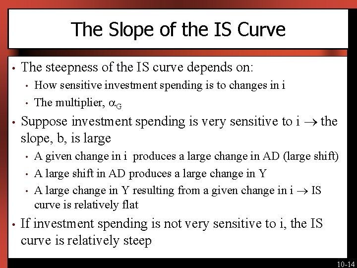
The Slope of the IS Curve • The steepness of the IS curve depends on: • • • Suppose investment spending is very sensitive to i the slope, b, is large • • How sensitive investment spending is to changes in i The multiplier, G A given change in i produces a large change in AD (large shift) A large shift in AD produces a large change in Y A large change in Y resulting from a given change in i IS curve is relatively flat If investment spending is not very sensitive to i, the IS curve is relatively steep 10 -14

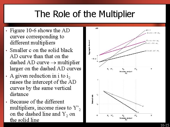
The Role of the Multiplier • • Figure 10 -6 shows the AD curves corresponding to different multipliers Smaller c on the solid black AD curve than that on the dashed AD curve multiplier larger on the dashed AD curves A given reduction in i to i 2 raises the intercept of the AD curves by the same vertical distance Because of the different multipliers, income rises to Y’ 2 on the dashed line and Y 2 on the solid line [Insert Figure 10 -6 here] 10 -15

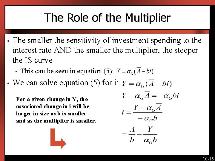
The Role of the Multiplier • The smaller the sensitivity of investment spending to the interest rate AND the smaller the multiplier, the steeper the IS curve • • This can be seen in equation (5): We can solve equation (5) for i: For a given change in Y, the associated change in i will be larger in size as b is smaller and as the multiplier is smaller. 10 -16

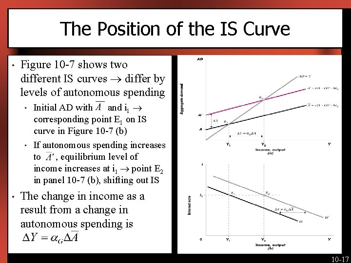
The Position of the IS Curve • Figure 10 -7 shows two different IS curves differ by levels of autonomous spending • • • [Insert Figure 10 -7 here] Initial AD with and i 1 corresponding point E 1 on IS curve in Figure 10 -7 (b) If autonomous spending increases to , equilibrium level of income increases at i 1 point E 2 in panel 10 -7 (b), shifting out IS The change in income as a result from a change in autonomous spending is 10 -17

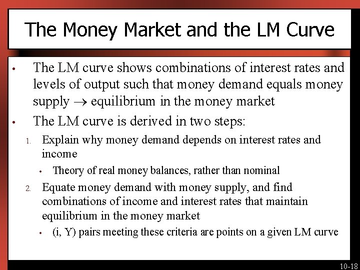
The Money Market and the LM Curve The LM curve shows combinations of interest rates and levels of output such that money demand equals money supply equilibrium in the money market The LM curve is derived in two steps: • • Explain why money demand depends on interest rates and income 1. • Theory of real money balances, rather than nominal Equate money demand with money supply, and find combinations of income and interest rates that maintain equilibrium in the money market 2. • (i, Y) pairs meeting these criteria are points on a given LM curve 10 -18

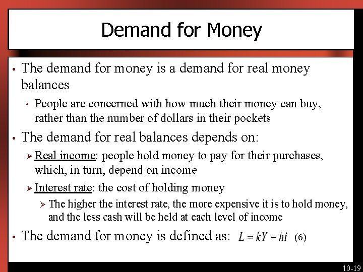
Demand for Money • The demand for money is a demand for real money balances • • People are concerned with how much their money can buy, rather than the number of dollars in their pockets The demand for real balances depends on: Ø Real income: people hold money to pay for their purchases, which, in turn, depend on income Ø Interest rate: the cost of holding money Ø • The higher the interest rate, the more expensive it is to hold money, and the less cash will be held at each level of income The demand for money is defined as: (6) 10 -19

Demand for Money (6) • • • [Insert Figure 10 -8 here] The parameters k and h reflect the sensitivity of the demand for real balances to the level of Y and i For a given level of income, the quantity demanded is a decreasing function of i Figure 10 -8 illustrates the inverse relationship between money demand i money demand curve 10 -20

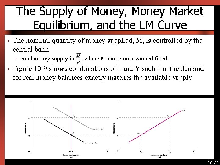
The Supply of Money, Money Market Equilibrium, and the LM Curve • The nominal quantity of money supplied, M, is controlled by the central bank • • Real money supply is , where M and P are assumed fixed Figure 10 -9 shows combinations of i and Y such that the demand for real money balances exactly matches the available supply [Insert Figure 10 -9 here] 10 -21

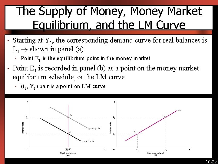
The Supply of Money, Money Market Equilibrium, and the LM Curve • Starting at Y 1, the corresponding demand curve for real balances is L 1 shown in panel (a) • • Point E 1 is the equilibrium point in the money market Point E 1 is recorded in panel (b) as a point on the money market equilibrium schedule, or the LM curve • (i 1, Y 1) pair is a point on LM curve [Insert Figure 10 -9 here] 10 -22

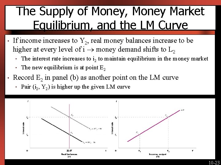
The Supply of Money, Money Market Equilibrium, and the LM Curve • If income increases to Y 2, real money balances increase to be higher at every level of i money demand shifts to L 2 • • • The interest rate increases to i 2 to maintain equilibrium in the money market The new equilibrium is at point E 2 Record E 2 in panel (b) as another point on the LM curve • Pair (i 2, Y 2) is higher up the given LM curve [Insert Figure 10 -9 here] 10 -23

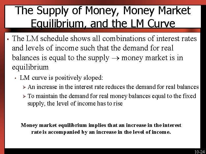
The Supply of Money, Money Market Equilibrium, and the LM Curve • The LM schedule shows all combinations of interest rates and levels of income such that the demand for real balances is equal to the supply money market is in equilibrium • LM curve is positively sloped: An increase in the interest rate reduces the demand for real balances Ø To maintain the demand for real money balances equal to the fixed supply, the level of income has to rise Ø Money market equilibrium implies that an increase in the interest rate is accompanied by an increase in the level of income. 10 -24

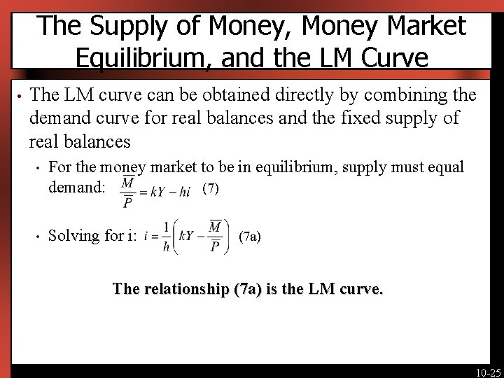
The Supply of Money, Money Market Equilibrium, and the LM Curve • The LM curve can be obtained directly by combining the demand curve for real balances and the fixed supply of real balances • For the money market to be in equilibrium, supply must equal demand: (7) • Solving for i: (7 a) The relationship (7 a) is the LM curve. 10 -25

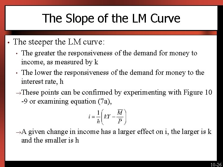
The Slope of the LM Curve • The steeper the LM curve: The greater the responsiveness of the demand for money to income, as measured by k • The lower the responsiveness of the demand for money to the interest rate, h These points can be confirmed by experimenting with Figure 10 -9 or examining equation (7 a), • A given change in income has a larger effect on i, the larger is k and the smaller is h 10 -26

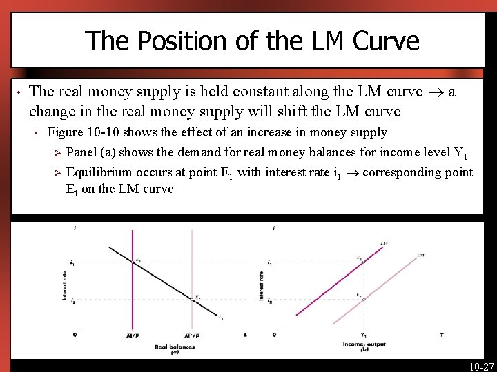
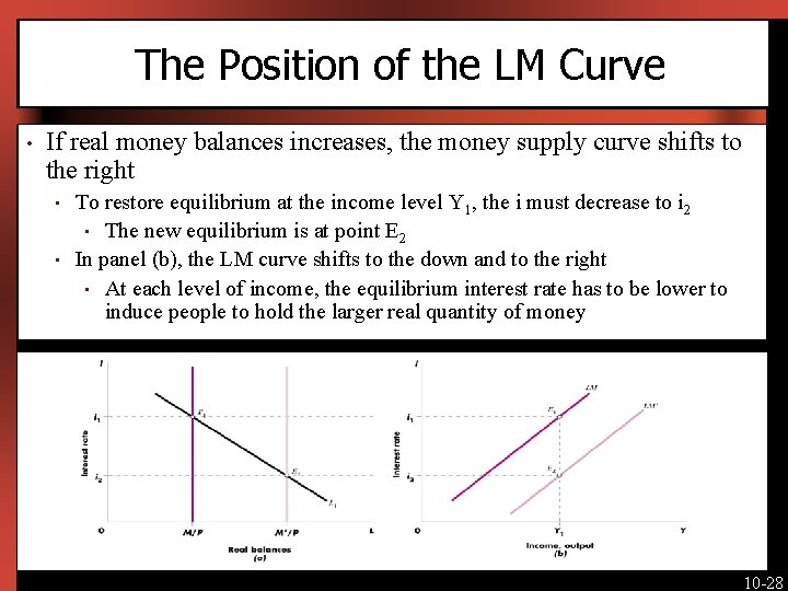
The Position of the LM Curve • The real money supply is held constant along the LM curve a change in the real money supply will shift the LM curve • Figure 10 -10 shows the effect of an increase in money supply Ø Panel (a) shows the demand for real money balances for income level Y 1 Ø Equilibrium occurs at point E 1 with interest rate i 1 corresponding point E 1 on the LM curve [Insert Figure 10 -10] 10 -27

The Position of the LM Curve • If real money balances increases, the money supply curve shifts to the right • • To restore equilibrium at the income level Y 1, the i must decrease to i 2 • The new equilibrium is at point E 2 In panel (b), the LM curve shifts to the down and to the right • At each level of income, the equilibrium interest rate has to be lower to induce people to hold the larger real quantity of money [Insert Figure 10 -10] 10 -28

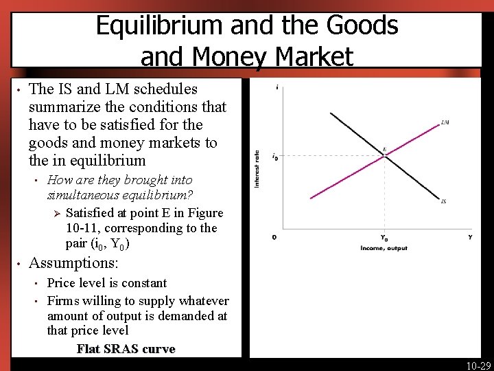
Equilibrium and the Goods and Money Market • The IS and LM schedules summarize the conditions that have to be satisfied for the goods and money markets to the in equilibrium • • [Insert Figure 10 -11 here] How are they brought into simultaneous equilibrium? Ø Satisfied at point E in Figure 10 -11, corresponding to the pair (i 0, Y 0) Assumptions: • • Price level is constant Firms willing to supply whatever amount of output is demanded at that price level Flat SRAS curve 10 -29

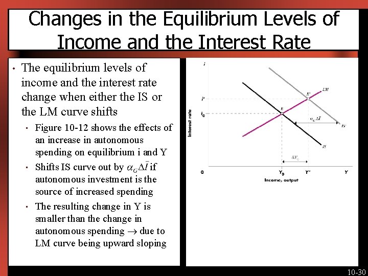
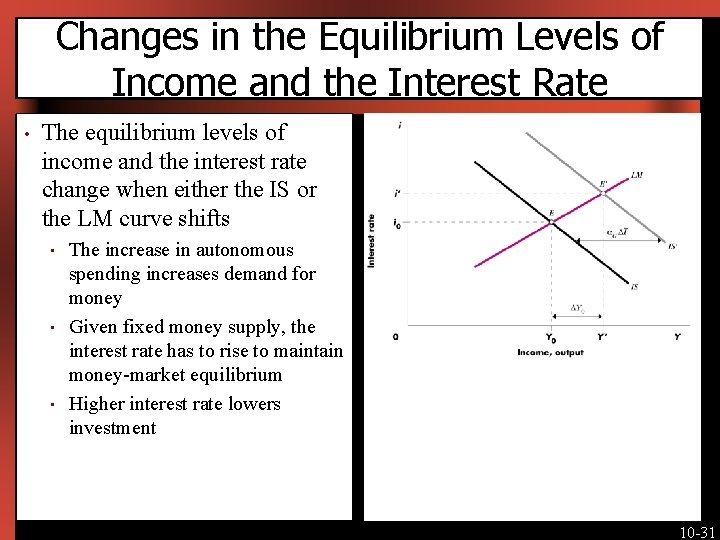
Changes in the Equilibrium Levels of Income and the Interest Rate • The equilibrium levels of income and the interest rate change when either the IS or the LM curve shifts • • • [Insert Figure 10 -12 here] Figure 10 -12 shows the effects of an increase in autonomous spending on equilibrium i and Y Shifts IS curve out by if autonomous investment is the source of increased spending The resulting change in Y is smaller than the change in autonomous spending due to LM curve being upward sloping 10 -30

Changes in the Equilibrium Levels of Income and the Interest Rate • The equilibrium levels of income and the interest rate change when either the IS or the LM curve shifts • • • [Insert Figure 10 -12 here] The increase in autonomous spending increases demand for money Given fixed money supply, the interest rate has to rise to maintain money-market equilibrium Higher interest rate lowers investment 10 -31

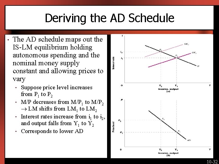
Deriving the AD Schedule • The AD schedule maps out the IS-LM equilibrium holding autonomous spending and the nominal money supply constant and allowing prices to vary • • [Insert Figure 10 -13 here] Suppose price level increases from P 1 to P 2 M/P decreases from M/P 1 to M/P 2 LM shifts from LM 1 to LM 2 Interest rates increase from i 1 to i 2, and output falls from Y 1 to Y 2 Corresponds to lower AD 10 -32

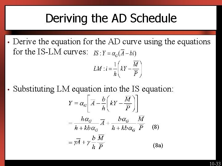
Deriving the AD Schedule • Derive the equation for the AD curve using the equations for the IS-LM curves: • Substituting LM equation into the IS equation: (8) (8 a) 10 -33

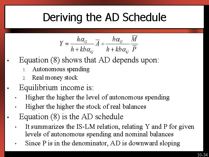
Deriving the AD Schedule Equation (8) shows that AD depends upon: • 1. 2. Autonomous spending Real money stock Equilibrium income is: • • • Higher the higher the level of autonomous spending Higher the higher the stock of real balances Equation (8) is the AD schedule • • • It summarizes the IS-LM relation, relating Y and P for given levels of autonomous spending and nominal balances Since P is in the denominator, AD is downward sloping 10 -34

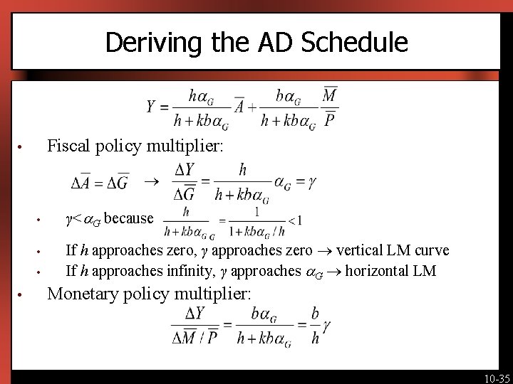
Deriving the AD Schedule Fiscal policy multiplier: • • • γ< G because If h approaches zero, γ approaches zero vertical LM curve If h approaches infinity, γ approaches G horizontal LM Monetary policy multiplier: 10 -35