Chapter 10 Logistic Regression Data Mining for Business

Chapter 10 – Logistic Regression Data Mining for Business Analytics Shmueli, Patel & Bruce

Logistic Regression Extends idea of linear regression to situation where outcome variable is categorical Widely used, particularly where a structured model is useful to classify (customers into returning or nonreturning) explain (profiling) – factors that differentiate predict class (approve or disapprove loan application) We focus on binary classification i. e. Y=0 or Y=1

The Logit Goal: Find a function of the predictor variables that relates them to a 0/1 outcome Instead of Y as outcome variable (like in linear regression), we use a function of Y called the logit Logit can be modeled as a linear function of the predictors The logit can be mapped back to a probability, which, in turn, can be mapped to a class

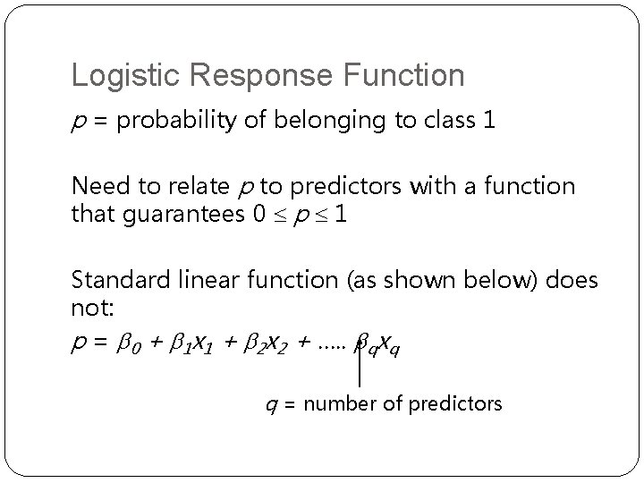
Logistic Response Function p = probability of belonging to class 1 Need to relate p to predictors with a function that guarantees 0 p 1 Standard linear function (as shown below) does not: p = b 0 + b 1 x 1 + b 2 x 2 + …. . bqxq q = number of predictors

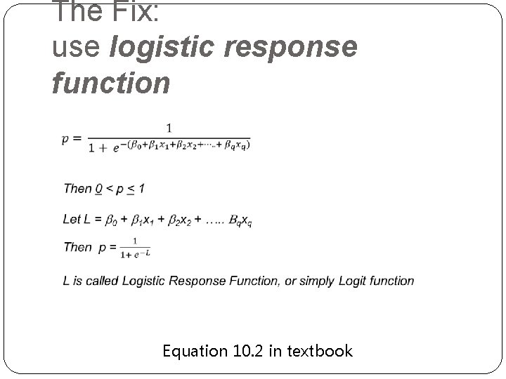
The Fix: use logistic response function Equation 10. 2 in textbook

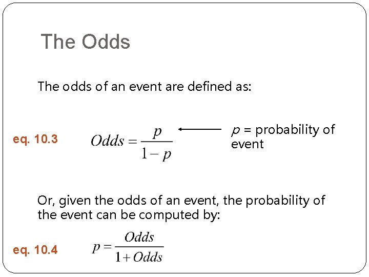
The Odds The odds of an event are defined as: eq. 10. 3 p = probability of event Or, given the odds of an event, the probability of the event can be computed by: eq. 10. 4

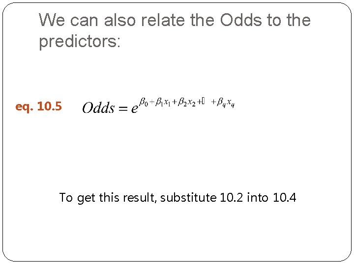
We can also relate the Odds to the predictors: eq. 10. 5 To get this result, substitute 10. 2 into 10. 4

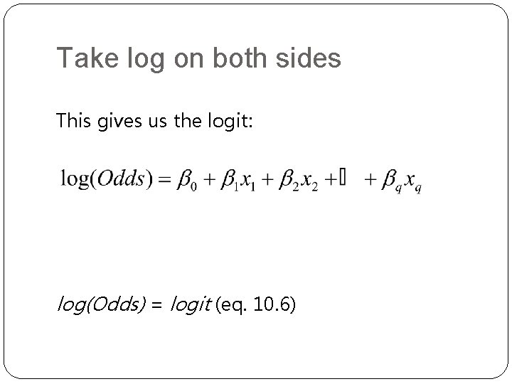
Take log on both sides This gives us the logit: log(Odds) = logit (eq. 10. 6)

Logit, cont. So, the logit is a linear function of predictors x 1, x 2, … Takes values from -infinity to +infinity Review the relationship between logit, odds and probability

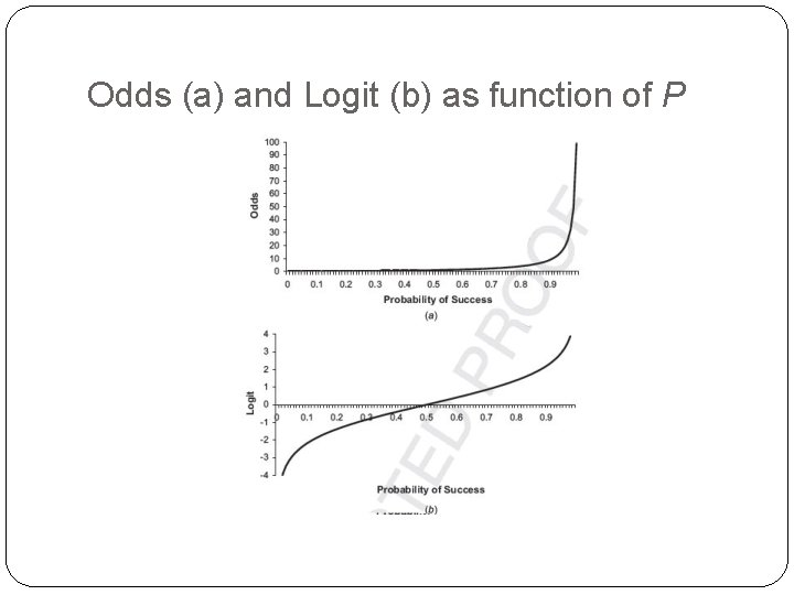
Odds (a) and Logit (b) as function of P

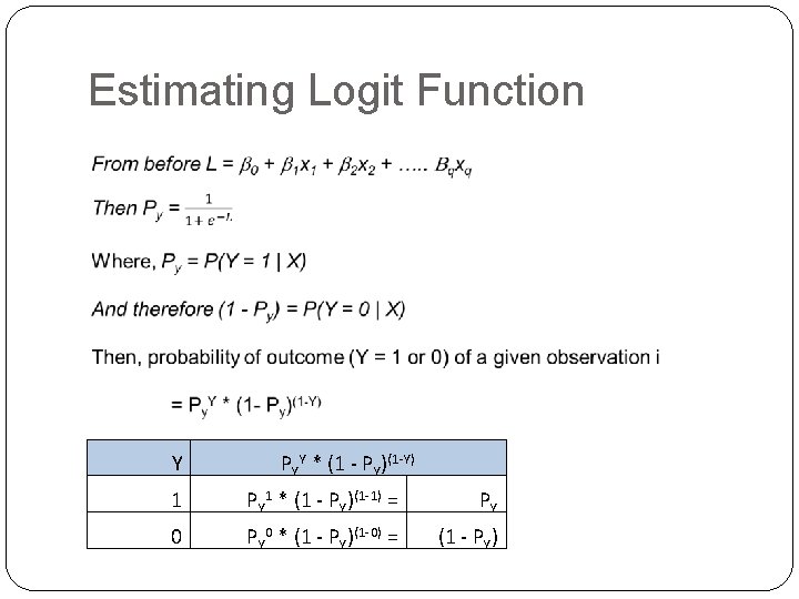
Estimating Logit Function Y PYY * (1 - PY)(1 -Y) 1 PY 1 * (1 - PY)(1 -1) = PY 0 * (1 - PY)(1 -0) = (1 - PY)

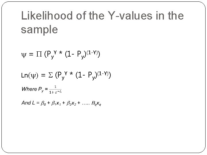
Likelihood of the Y-values in the sample y = P (Py. Y * (1 - Py)(1 -Y)) Ln(y) = S (Py. Y * (1 - Py)(1 -Y))

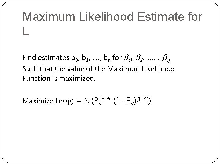
Maximum Likelihood Estimate for L Find estimates b 0, b 1, …. , bq for b 0, b 1, …. , bq Such that the value of the Maximum Likelihood Function is maximized. Maximize Ln(y) = S (Py. Y * (1 - Py)(1 -Y))

Example

Personal Loan Offer Outcome variable: accept bank loan (0/1) Predictors: Demographic info, and info about their bank relationship

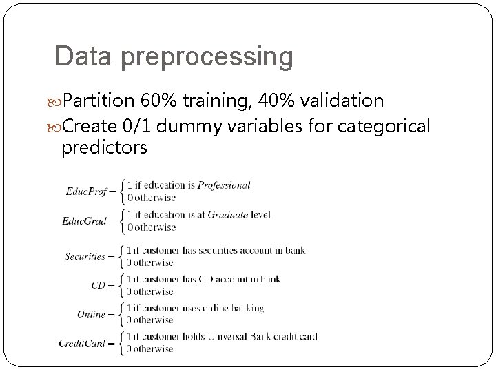
Data preprocessing Partition 60% training, 40% validation Create 0/1 dummy variables for categorical predictors

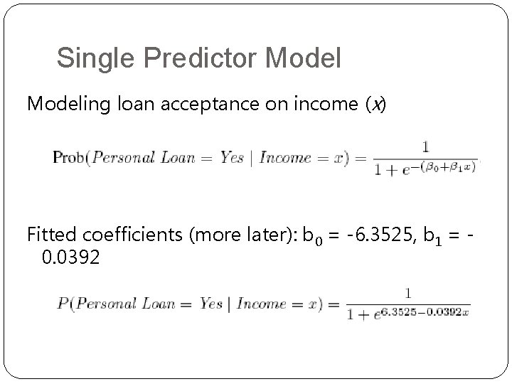
Single Predictor Modeling loan acceptance on income (x) Fitted coefficients (more later): b 0 = -6. 3525, b 1 = 0. 0392

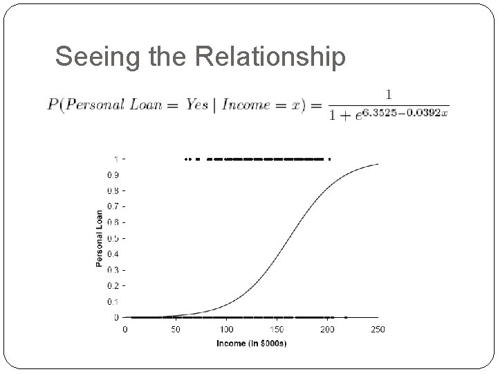
Seeing the Relationship

Last step - classify Model produces an estimated probability of being a “ 1” Convert to a classification by establishing cutoff level If estimated prob. > cutoff, classify as “ 1”

Ways to Determine Cutoff 0. 50 is popular initial choice Additional considerations (see Chapter 5) Maximize classification accuracy Maximize sensitivity (subject to min. level of specificity) Minimize false positives (subject to max. false negative rate) Minimize expected cost of misclassification (need to specify costs)

Example, cont. Estimates of b’s are derived through an iterative process called maximum likelihood estimation Let’s include all 12 predictors in the model now XLMiner’s output gives coefficients for the logit, as well as odds for the individual terms

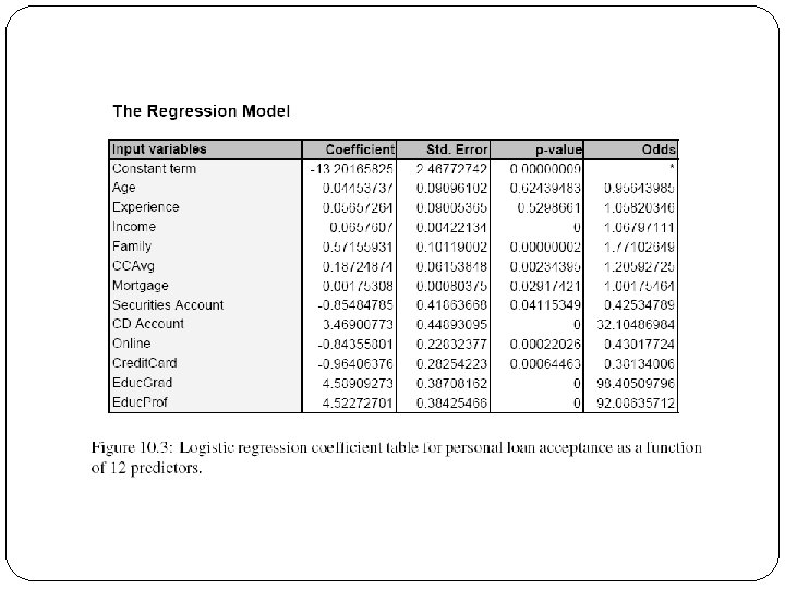
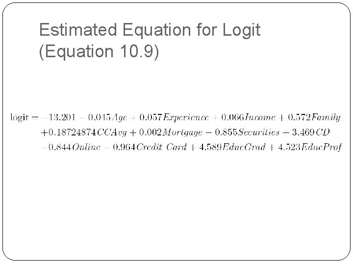
Estimated Equation for Logit (Equation 10. 9)

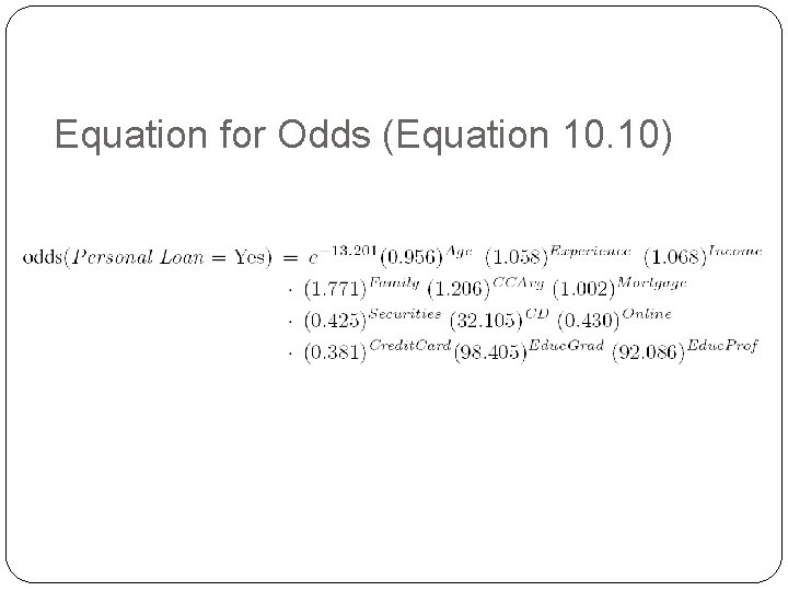
Equation for Odds (Equation 10. 10)

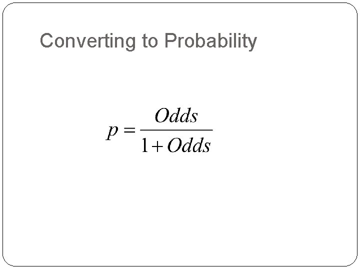
Converting to Probability

Interpreting Odds, Probability For predictive classification, we typically use probability with a cutoff value For explanatory purposes, odds have a useful interpretation: If we increase x 1 by one unit, holding x 2, x 3 … xq constant, then b 1 is the factor by which the odds of belonging to class 1 increase

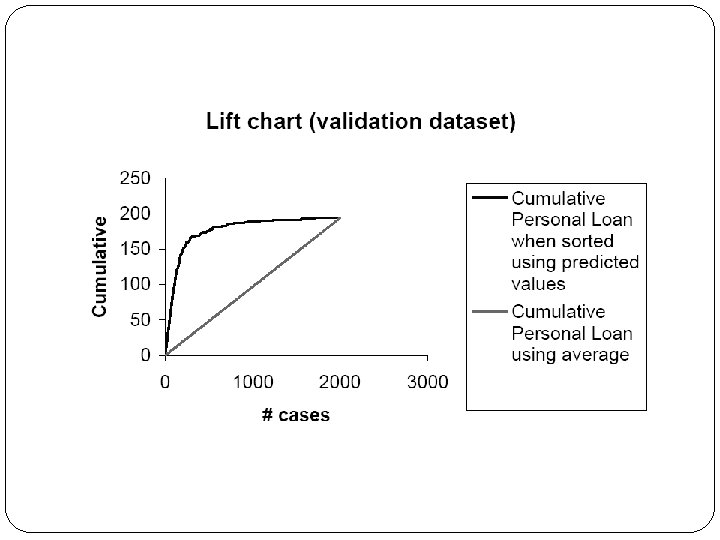
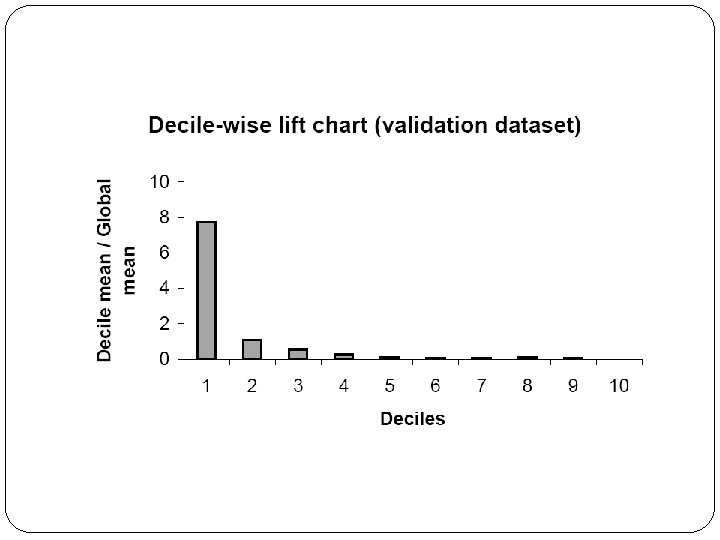
Loan Example: Evaluating Classification Performance measures: Confusion matrix and % of misclassifications More useful in this example: lift

Multicollinearity Problem: As in linear regression, if one predictor is a linear combination of other predictor(s), model estimation will fail Note that in such a case, we have at least one redundant predictor Solution: Remove extreme redundancies (by dropping predictors via variable selection – see next, or by data reduction methods such as PCA)

Variable Selection This is the same issue as in linear regression The number of correlated predictors can grow when we create derived variables such as interaction terms (e. g. Income x Family), to capture more complex relationships Problem: Overly complex models have the danger of overfitting Solution: Reduce variables via automated selection of variable subsets (as with linear regression)

P-values for Predictors Test null hypothesis that coefficient = 0 Useful for review to determine whether to include variable in model Key in profiling tasks, but less important in predictive classification

Complete Example: Predicting Delayed Flights DC to NY

Variables Outcome: delayed or not-delayed Predictors: Day of week Departure time Origin (DCA, IAD, BWI) Destination (LGA, JFK, EWR) Carrier Weather (1 = bad weather)

Data Preprocessing Create binary dummies for the categorical variables Partition 60%-40% into training/validation

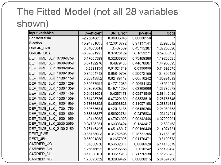
The Fitted Model (not all 28 variables shown)

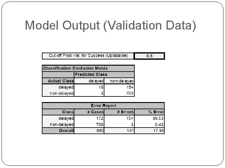
Model Output (Validation Data)

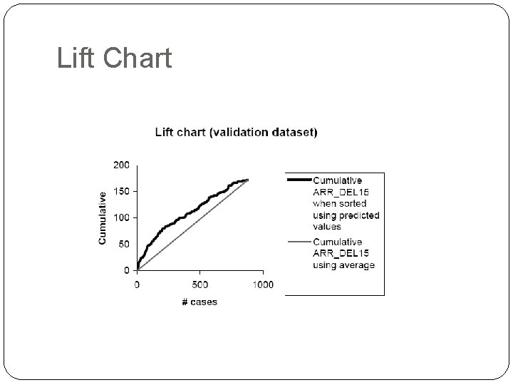
Lift Chart

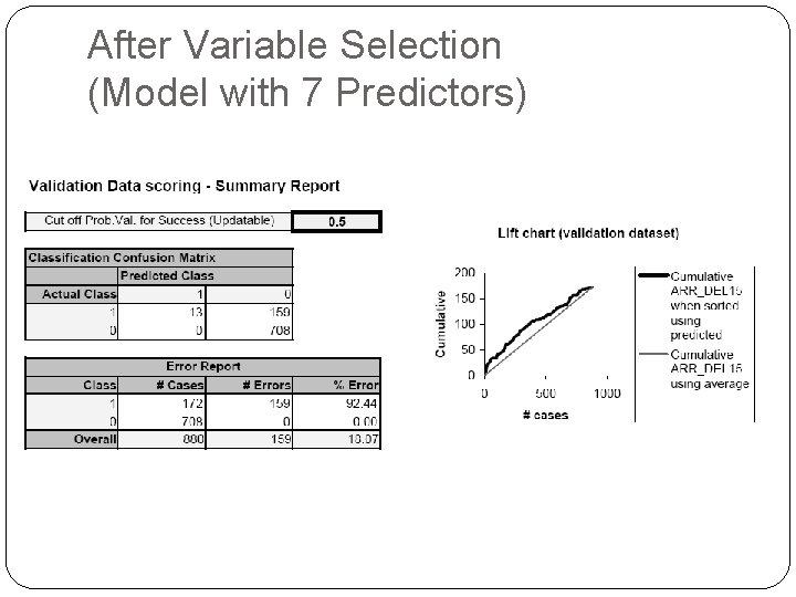
After Variable Selection (Model with 7 Predictors)

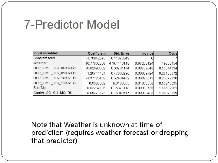
7 -Predictor Model Note that Weather is unknown at time of prediction (requires weather forecast or dropping that predictor)

Summary Logistic regression is similar to linear regression, except that it is used with a categorical response It can be used for explanatory tasks (=profiling) or predictive tasks (=classification) The predictors are related to the response Y via a nonlinear function called the logit As in linear regression, reducing predictors can be done via variable selection Logistic regression can be generalized to more than two classes (not in XLMiner)