Chapter 10 Introduction to Data Mining Data Mining

Chapter 10 Introduction to Data Mining

Data Mining Data mining is focused on better understanding of characteristics and patterns among variables in large databases using a variety of statistical and analytical tools. ◦ It is used to identify relationships among variables in large data sets and understand hidden patterns that they may contain. ◦ XLMiner software implement many basic data mining procedures in a spreadsheet environment.

The Scope of Data Mining � Data Exploration and Reduction �identifying groups in which elements are in some way similar � Classification �analyzing data to predict how to classify a new data element � Association �analyzing databases to identify natural associations among variables and create rules for target marketing or buying recommendations � Cause-and-effect Modeling �developing analytic models to describe relationships between metrics that drive business performance

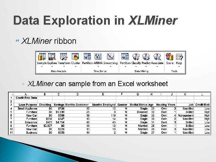
Data Exploration in XLMiner ribbon ◦ XLMiner can sample from an Excel worksheet

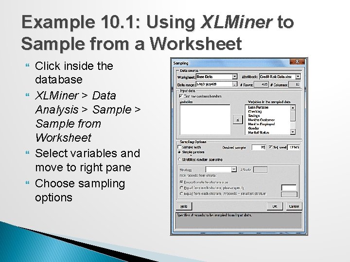
Example 10. 1: Using XLMiner to Sample from a Worksheet Click inside the database XLMiner > Data Analysis > Sample from Worksheet Select variables and move to right pane Choose sampling options

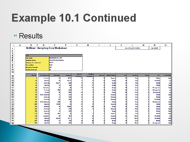
Example 10. 1 Continued Results

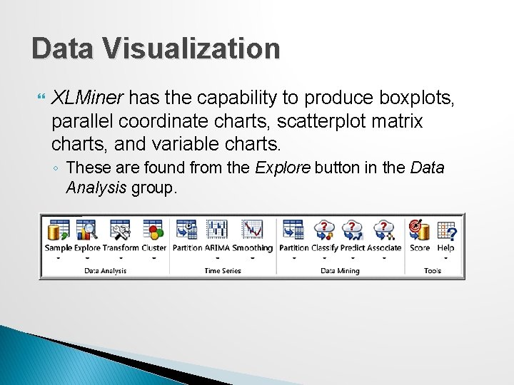
Data Visualization XLMiner has the capability to produce boxplots, parallel coordinate charts, scatterplot matrix charts, and variable charts. ◦ These are found from the Explore button in the Data Analysis group.

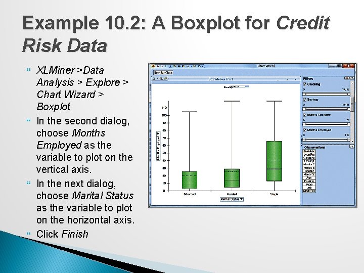
Example 10. 2: A Boxplot for Credit Risk Data XLMiner >Data Analysis > Explore > Chart Wizard > Boxplot In the second dialog, choose Months Employed as the variable to plot on the vertical axis. In the next dialog, choose Marital Status as the variable to plot on the horizontal axis. Click Finish

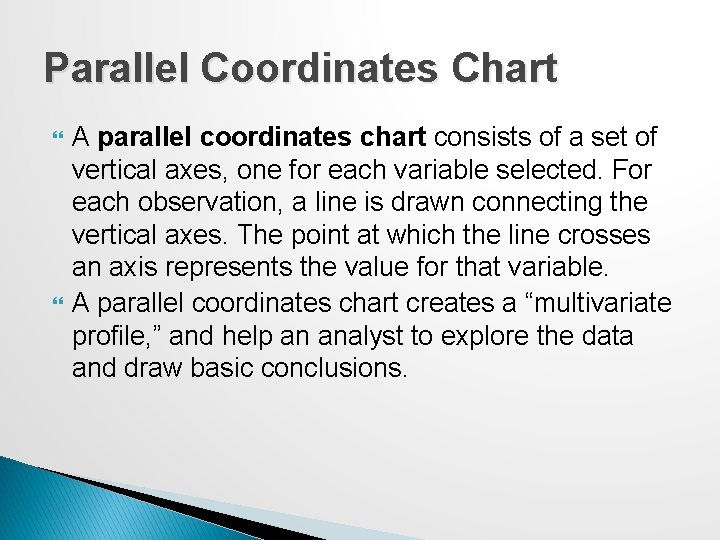
Parallel Coordinates Chart A parallel coordinates chart consists of a set of vertical axes, one for each variable selected. For each observation, a line is drawn connecting the vertical axes. The point at which the line crosses an axis represents the value for that variable. A parallel coordinates chart creates a “multivariate profile, ” and help an analyst to explore the data and draw basic conclusions.

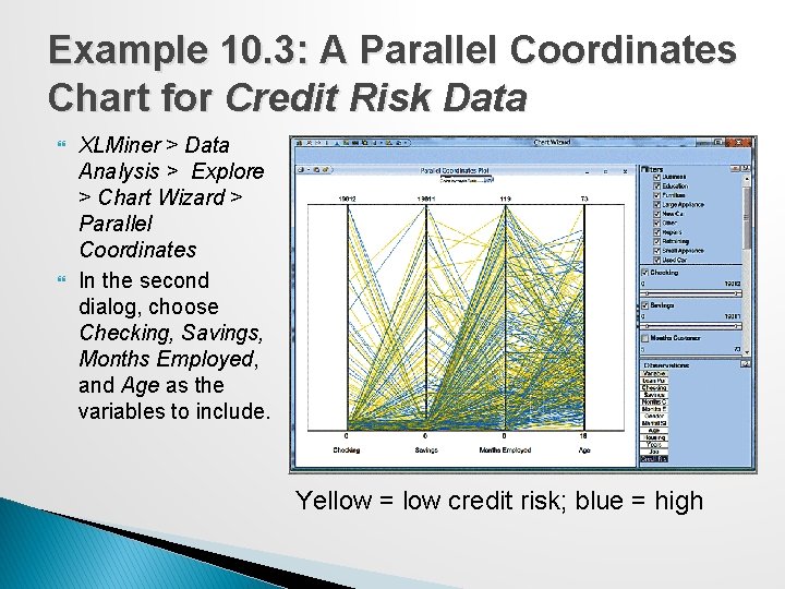
Example 10. 3: A Parallel Coordinates Chart for Credit Risk Data XLMiner > Data Analysis > Explore > Chart Wizard > Parallel Coordinates In the second dialog, choose Checking, Savings, Months Employed, and Age as the variables to include. Yellow = low credit risk; blue = high

Scatterplot Matrix A scatterplot matrix combines several scatter charts into one panel, allowing the user to visualize pairwise relationships between variables.

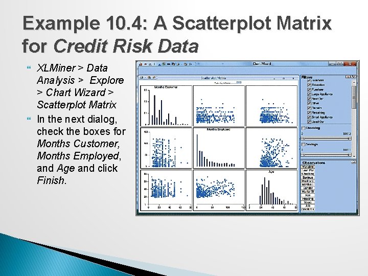
Example 10. 4: A Scatterplot Matrix for Credit Risk Data XLMiner > Data Analysis > Explore > Chart Wizard > Scatterplot Matrix In the next dialog, check the boxes for Months Customer, Months Employed, and Age and click Finish.

Variable Plot A variable plots a matrix of histograms for the variables selected.

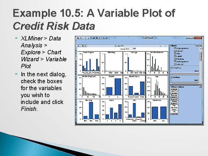
Example 10. 5: A Variable Plot of Credit Risk Data XLMiner > Data Analysis > Explore > Chart Wizard > Variable Plot In the next dialog, check the boxes for the variables you wish to include and click Finish.

Dirty Data Real data sets that have missing values or errors. Such data sets are called “dirty” and need to be “cleaned” prior to analyzing them. Approaches for handling missing data. ◦ Eliminate the records that contain missing data ◦ Estimate reasonable values for missing observations, such as the mean or median value ◦ Use a data mining procedure to deal with them. XLMiner has the capability to deal with missing data in the Transform menu in the Data Analysis group. Try to understand whether missing data are simply random events or if there is a logical reason. Eliminating sample data indiscriminately could result in misleading information and conclusions about the data.

Cluster Analysis Cluster analysis, also called data segmentation, is a collection of techniques that seek to group or segment a collection of objects (observations or records) into subsets or clusters, such that those within each cluster are more closely related to one another than objects assigned to different clusters. ◦ The objects within clusters should exhibit a high amount of similarity, whereas those in different clusters will be dissimilar.

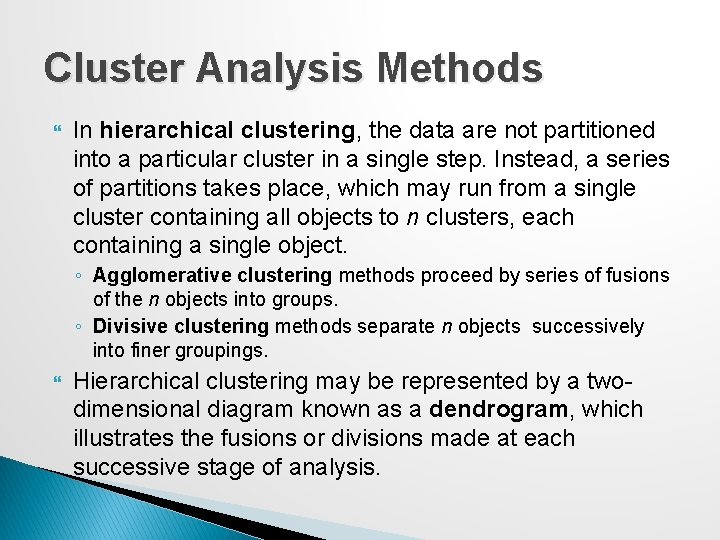
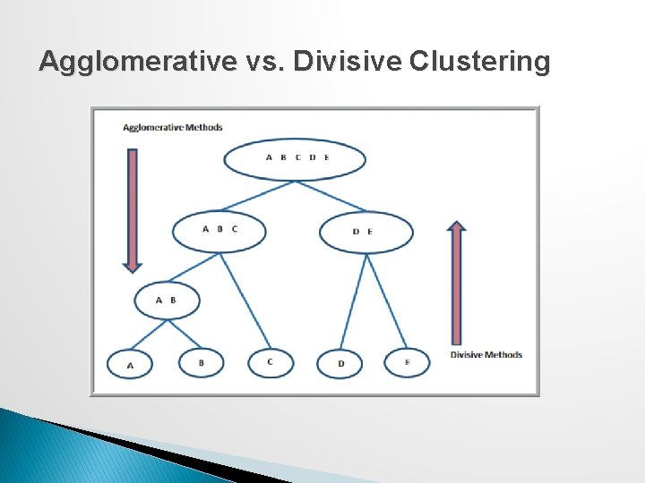
Cluster Analysis Methods In hierarchical clustering, the data are not partitioned into a particular cluster in a single step. Instead, a series of partitions takes place, which may run from a single cluster containing all objects to n clusters, each containing a single object. ◦ Agglomerative clustering methods proceed by series of fusions of the n objects into groups. ◦ Divisive clustering methods separate n objects successively into finer groupings. Hierarchical clustering may be represented by a twodimensional diagram known as a dendrogram, which illustrates the fusions or divisions made at each successive stage of analysis.

Agglomerative vs. Divisive Clustering

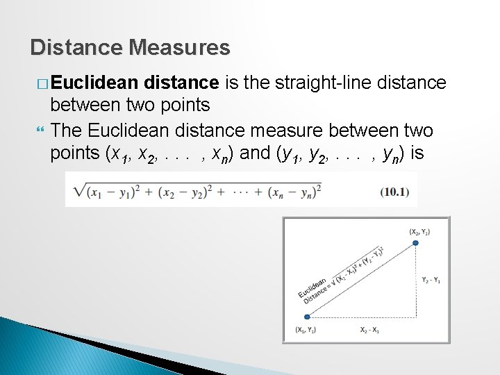
Distance Measures � Euclidean distance is the straight-line distance between two points The Euclidean distance measure between two points (x 1, x 2, . . . , xn) and (y 1, y 2, . . . , yn) is

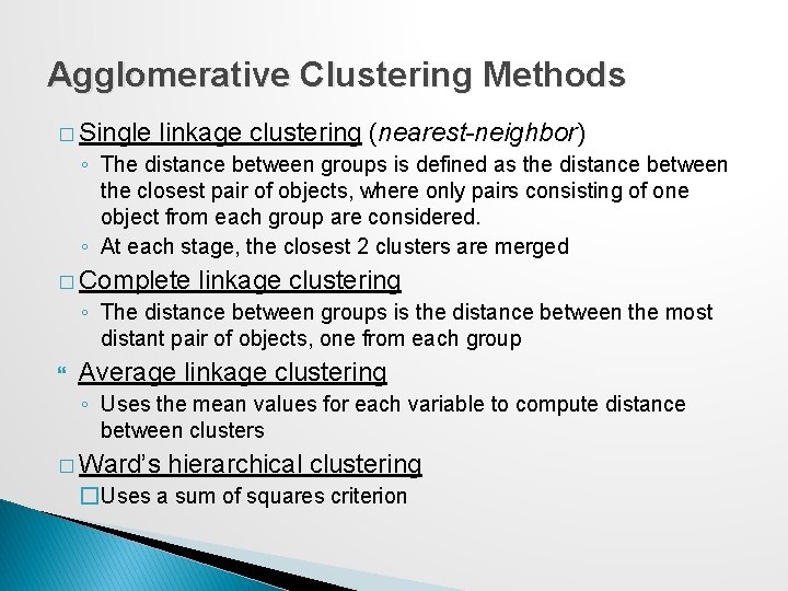
Agglomerative Clustering Methods � Single linkage clustering (nearest-neighbor) ◦ The distance between groups is defined as the distance between the closest pair of objects, where only pairs consisting of one object from each group are considered. ◦ At each stage, the closest 2 clusters are merged � Complete linkage clustering ◦ The distance between groups is the distance between the most distant pair of objects, one from each group Average linkage clustering ◦ Uses the mean values for each variable to compute distance between clusters � Ward’s hierarchical clustering �Uses a sum of squares criterion

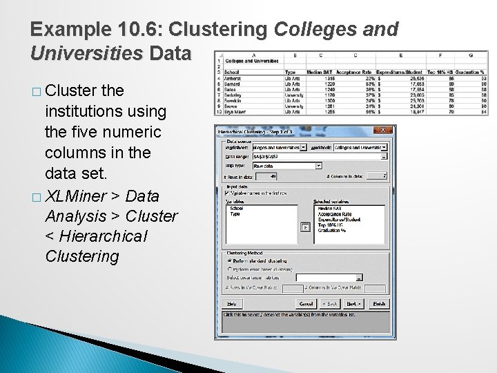
Example 10. 6: Clustering Colleges and Universities Data � Cluster the institutions using the five numeric columns in the data set. � XLMiner > Data Analysis > Cluster < Hierarchical Clustering

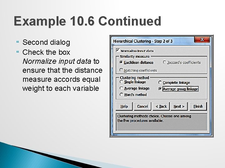
Example 10. 6 Continued Second dialog Check the box Normalize input data to ensure that the distance measure accords equal weight to each variable

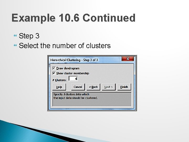
Example 10. 6 Continued Step 3 Select the number of clusters

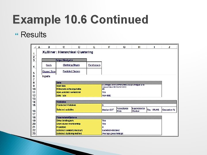
Example 10. 6 Continued Results

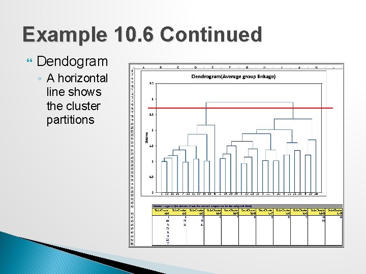
Example 10. 6 Continued Dendogram ◦ A horizontal line shows the cluster partitions

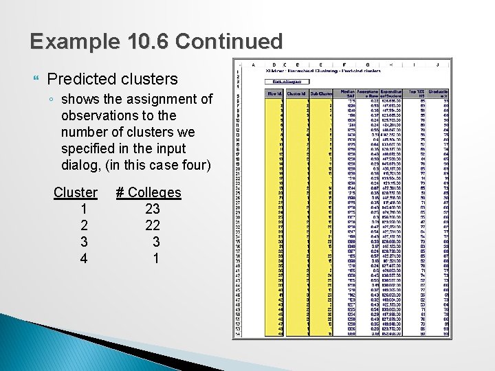
Example 10. 6 Continued Predicted clusters ◦ shows the assignment of observations to the number of clusters we specified in the input dialog, (in this case four) Cluster 1 2 3 4 # Colleges 23 22 3 1

Classification Classification methods seek to classify a categorical outcome into one of two or more categories based on various data attributes. For each record in a database, we have a categorical variable of interest and a number of additional predictor variables. For a given set of predictor variables, we would like to assign the best value of the categorical variable.

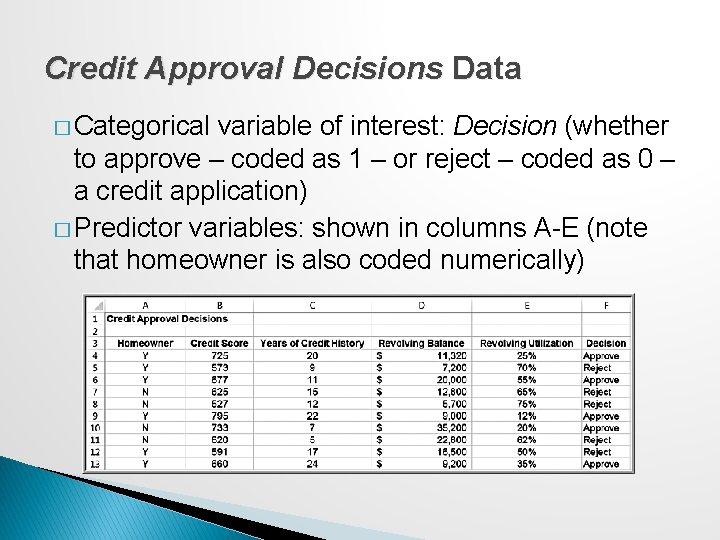
Credit Approval Decisions Data � Categorical variable of interest: Decision (whether to approve – coded as 1 – or reject – coded as 0 – a credit application) � Predictor variables: shown in columns A-E (note that homeowner is also coded numerically)

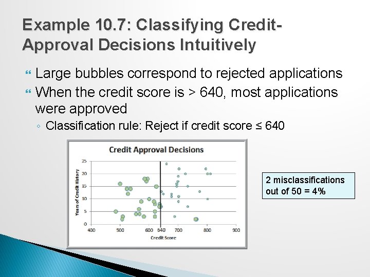
Example 10. 7: Classifying Credit. Approval Decisions Intuitively Large bubbles correspond to rejected applications When the credit score is > 640, most applications were approved ◦ Classification rule: Reject if credit score ≤ 640 2 misclassifications out of 50 = 4%

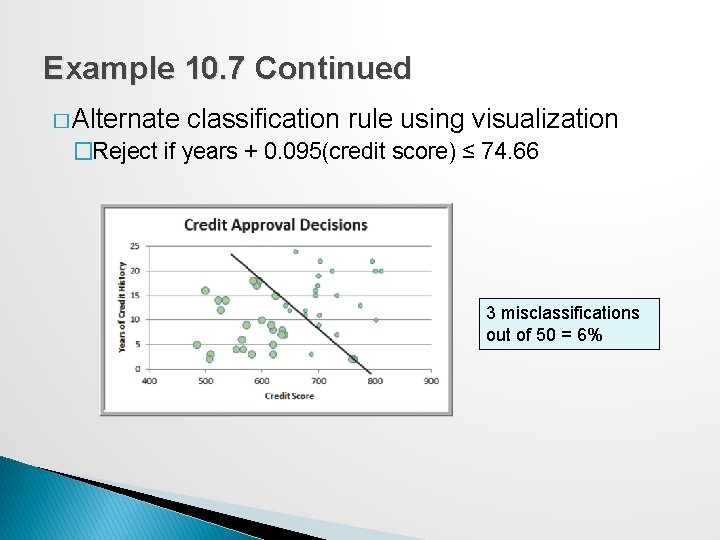
Example 10. 7 Continued � Alternate classification rule using visualization �Reject if years + 0. 095(credit score) ≤ 74. 66 3 misclassifications out of 50 = 6%

Measuring Classification Performance Find the probability of making a misclassification error and summarize the results in a classification matrix, which shows the number of cases that were classified either correctly or incorrectly.

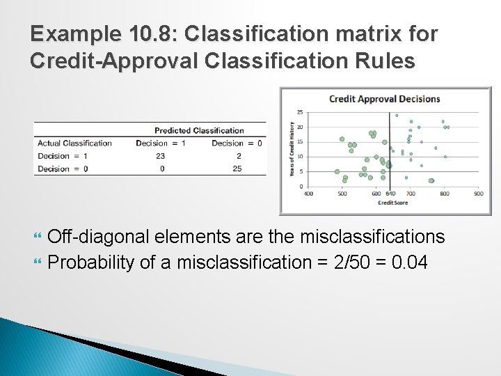
Example 10. 8: Classification matrix for Credit-Approval Classification Rules Off-diagonal elements are the misclassifications Probability of a misclassification = 2/50 = 0. 04

Using Training and Validation Data � Data mining projects typically involve large volumes of data. � The data can be partitioned into: ▪ training data set – has known outcomes and is used to “teach” the data-mining algorithm ▪ validation data set – used to fine-tune a model ▪ test data set – tests the accuracy of the model � In XLMiner, partitioning can be random or userspecified.

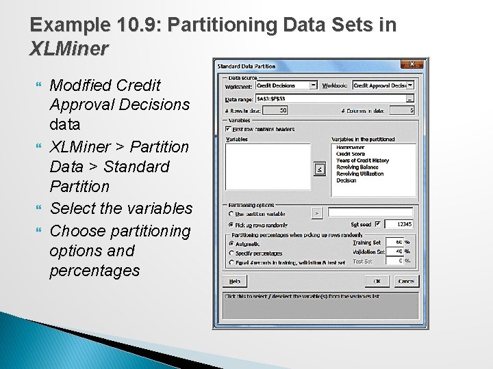
Example 10. 9: Partitioning Data Sets in XLMiner Modified Credit Approval Decisions data XLMiner > Partition Data > Standard Partition Select the variables Choose partitioning options and percentages

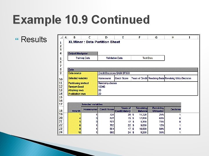
Example 10. 9 Continued Results

Classifying New Data After a classification scheme is chosen and the best model is developed based on existing data, we use the predictor variables as inputs to the model to predict the output.

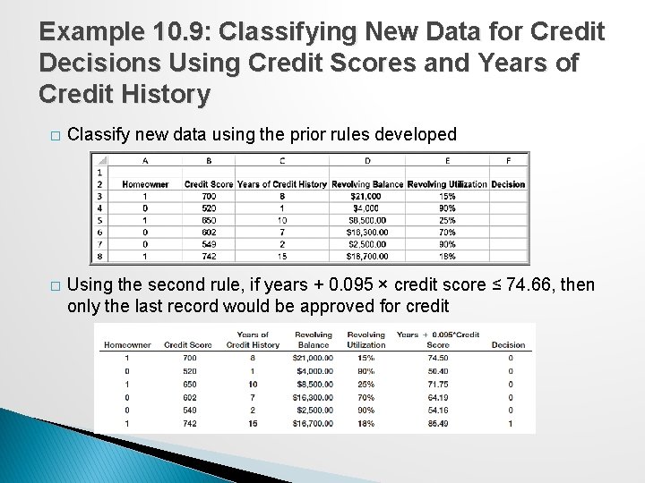
Example 10. 9: Classifying New Data for Credit Decisions Using Credit Scores and Years of Credit History � Classify new data using the prior rules developed � Using the second rule, if years + 0. 095 × credit score ≤ 74. 66, then only the last record would be approved for credit

Classification Techniques k-Nearest Neighbors (k-NN) Algorithm Finds records in a database that have similar numerical values of a set of predictor variables Discriminant Analysis Uses predefined classes based on a set of linear discriminant functions of the predictor variables Logistic Regression Estimates the probability of belonging to a category using a regression on the predictor variables

k-Nearest Neighbors (k-NN) Measure the Euclidean distance between records in the training data set. The nearest neighbor to a record in the training data set is the one that has the smallest distance from it. ◦ If k = 1, then the 1 -NN rule classifies a record in the same category as its nearest neighbor. ◦ k-NN rule finds the k-Nearest Neighbors in the training data set to each record we want to classify and then assigns the classification as the classification of majority of the k nearest neighbors Typically, various values of k are used and then results inspected to determine which is best.

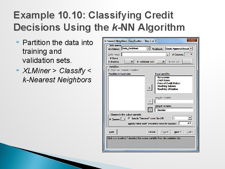
Example 10. 10: Classifying Credit Decisions Using the k-NN Algorithm Partition the data into training and validation sets. XLMiner > Classify < k-Nearest Neighbors

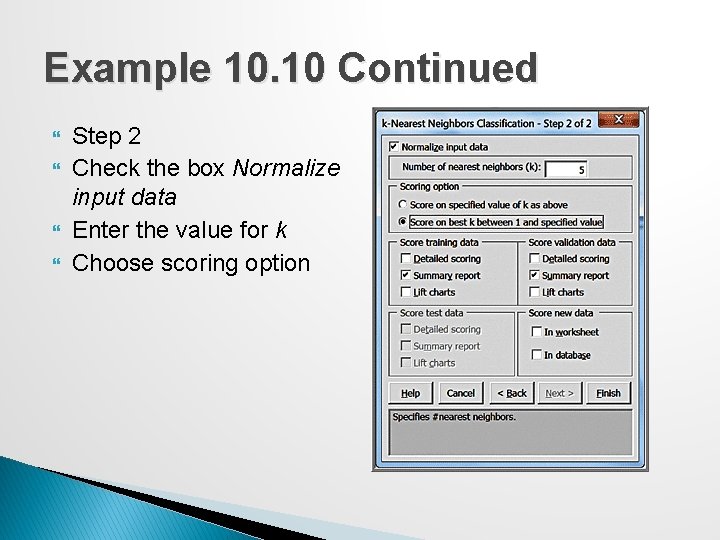
Example 10. 10 Continued Step 2 Check the box Normalize input data Enter the value for k Choose scoring option

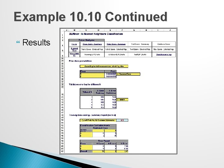
Example 10. 10 Continued Results

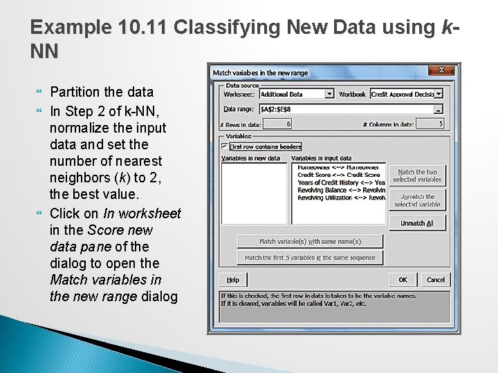
Example 10. 11 Classifying New Data using k. NN Partition the data In Step 2 of k-NN, normalize the input data and set the number of nearest neighbors (k) to 2, the best value. Click on In worksheet in the Score new data pane of the dialog to open the Match variables in the new range dialog

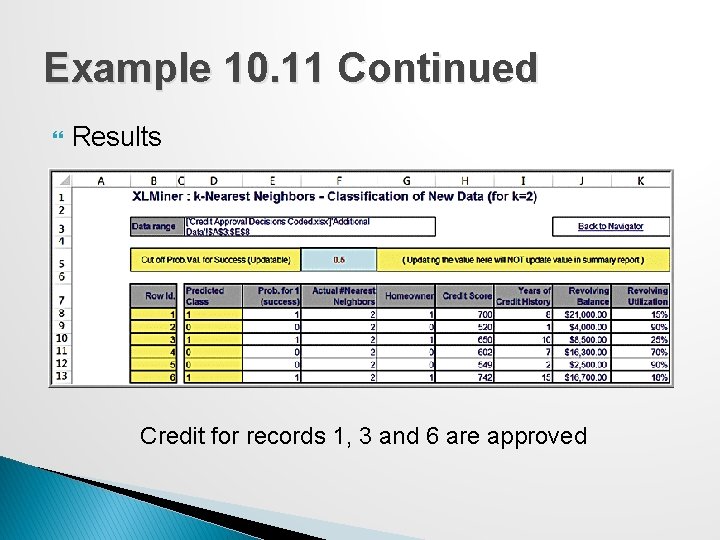
Example 10. 11 Continued Results Credit for records 1, 3 and 6 are approved

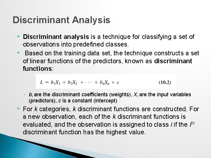
Discriminant Analysis Discriminant analysis is a technique for classifying a set of observations into predefined classes. Based on the training data set, the technique constructs a set of linear functions of the predictors, known as discriminant functions: ◦ bi are the discriminant coefficients (weights), Xi are the input variables (predictors), c is a constant (intercept) For k categories, k discriminant functions are constructed. For a new observation, each of the k discriminant functions is evaluated, and the observation is assigned to class i if the ith discriminant function has the highest value.

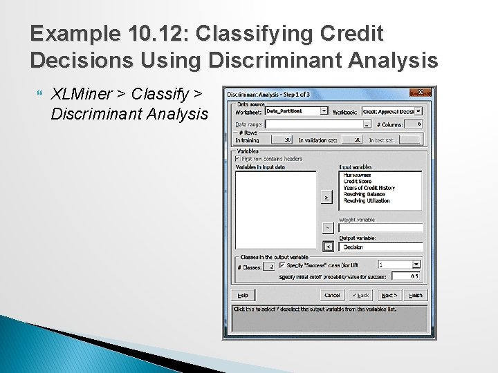
Example 10. 12: Classifying Credit Decisions Using Discriminant Analysis XLMiner > Classify > Discriminant Analysis

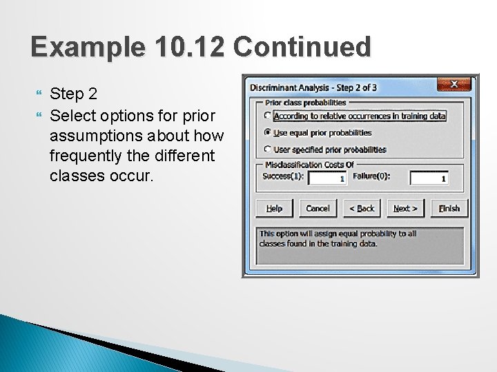
Example 10. 12 Continued Step 2 Select options for prior assumptions about how frequently the different classes occur.

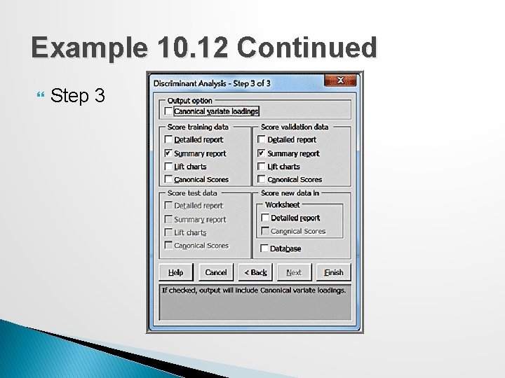
Example 10. 12 Continued Step 3

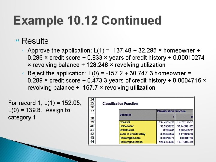
Example 10. 12 Continued Results ◦ Approve the application: L(1) = -137. 48 + 32. 295 × homeowner + 0. 286 × credit score + 0. 833 × years of credit history + 0. 00010274 × revolving balance + 128. 248 × revolving utilization ◦ Reject the application: L(0) = -157. 2 + 30. 747 3 homeowner = 0. 289 × credit score + 0. 473 3 years of credit history + 0. 0004716 × revolving balance + 167. 7 × revolving utilization For record 1, L(1) = 152. 05; L(0) = 139. 8. Assign to category 1

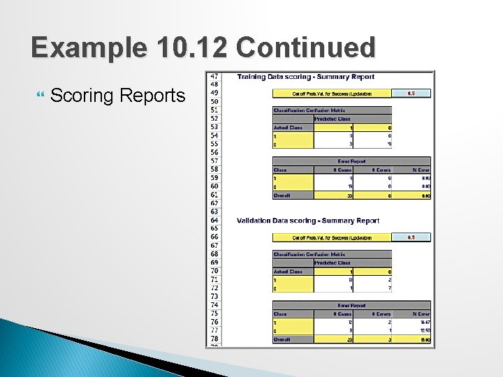
Example 10. 12 Continued Scoring Reports

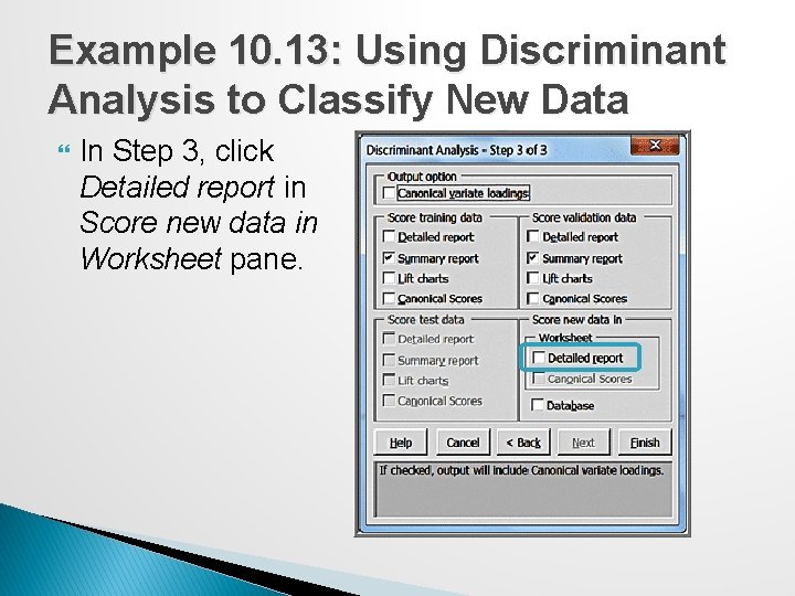
Example 10. 13: Using Discriminant Analysis to Classify New Data In Step 3, click Detailed report in Score new data in Worksheet pane.

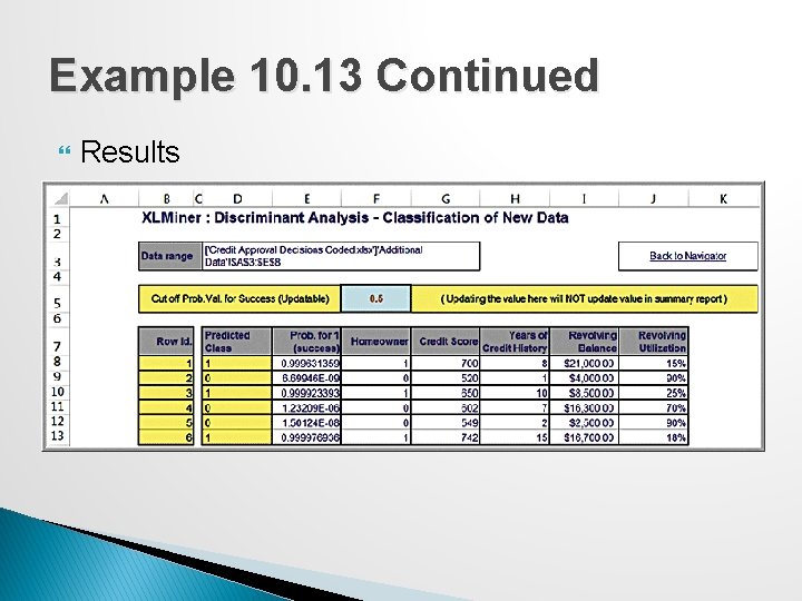
Example 10. 13 Continued Results

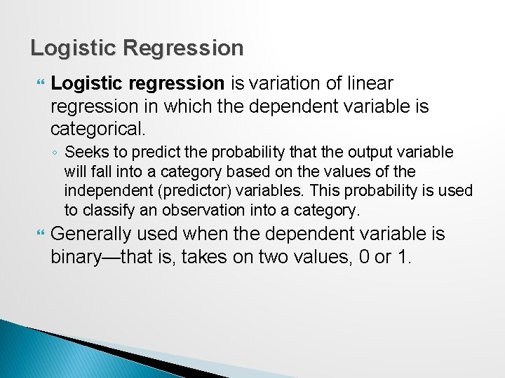
Logistic Regression Logistic regression is variation of linear regression in which the dependent variable is categorical. ◦ Seeks to predict the probability that the output variable will fall into a category based on the values of the independent (predictor) variables. This probability is used to classify an observation into a category. Generally used when the dependent variable is binary—that is, takes on two values, 0 or 1.

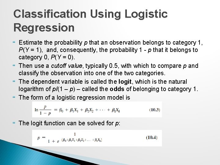
Classification Using Logistic Regression Estimate the probability p that an observation belongs to category 1, P(Y = 1), and, consequently, the probability 1 - p that it belongs to category 0, P(Y = 0). Then use a cutoff value, typically 0. 5, with which to compare p and classify the observation into one of the two categories. The dependent variable is called the logit, which is the natural logarithm of p/(1 – p) – called the odds of belonging to category 1. The form of a logistic regression model is The logit function can be solved for p:

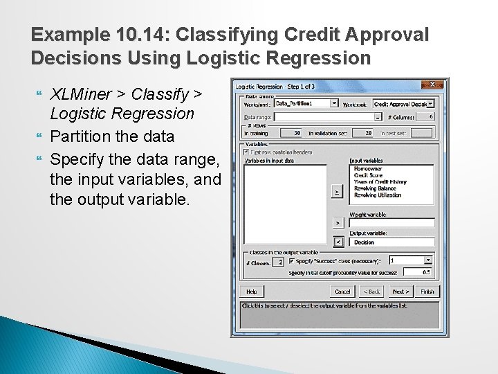
Example 10. 14: Classifying Credit Approval Decisions Using Logistic Regression XLMiner > Classify > Logistic Regression Partition the data Specify the data range, the input variables, and the output variable.

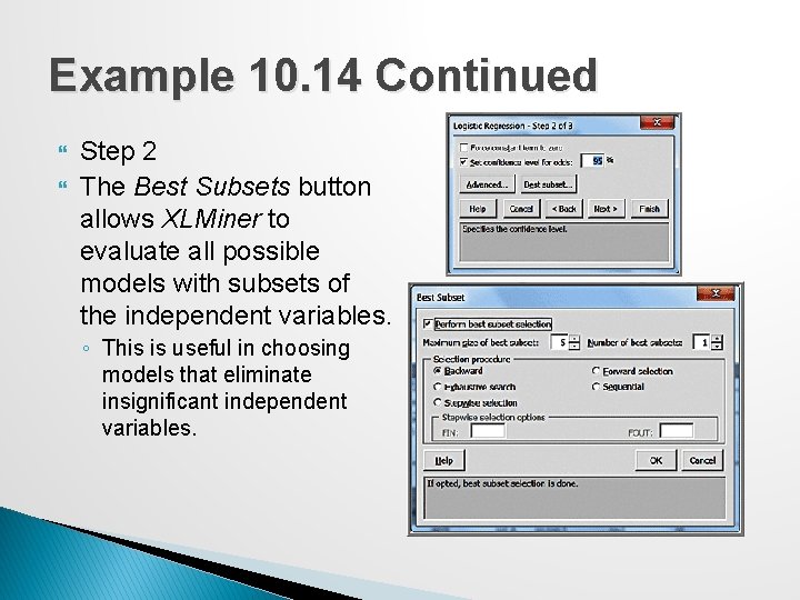
Example 10. 14 Continued Step 2 The Best Subsets button allows XLMiner to evaluate all possible models with subsets of the independent variables. ◦ This is useful in choosing models that eliminate insignificant independent variables.

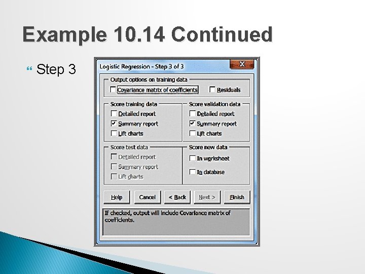
Example 10. 14 Continued Step 3

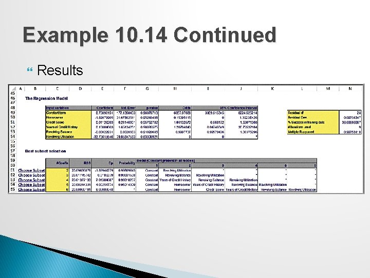
Example 10. 14 Continued Results

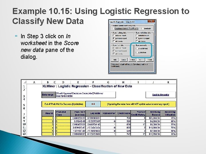
Example 10. 15: Using Logistic Regression to Classify New Data In Step 3 click on In worksheet in the Score new data pane of the dialog.

Association Rule Mining Association rule mining, often called affinity analysis, seeks to uncover associations and/or correlationships in large data sets ◦ Association rules identify attributes that occur together frequently in a given data set. ◦ Market basket analysis, for example, is used determine groups of items consumers tend to purchase together. Association rules provide information in the form of if-then (antecedent-consequent) statements.

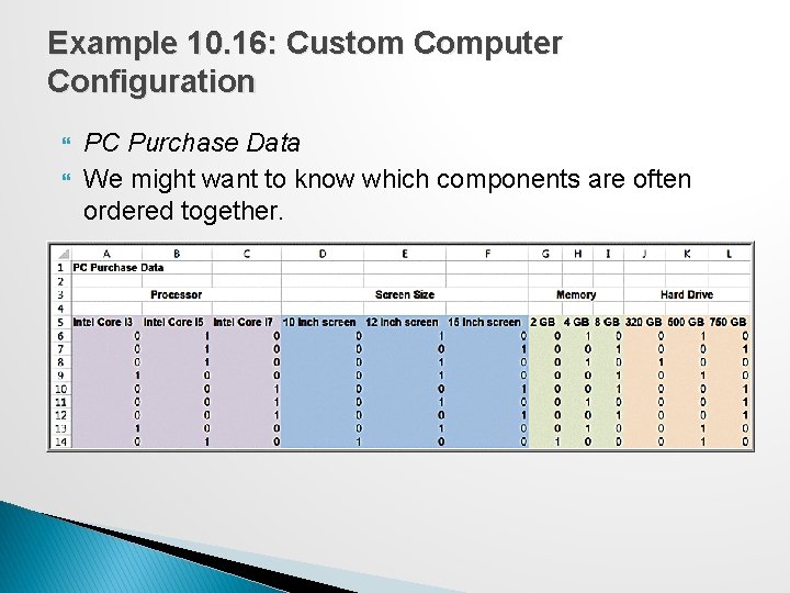
Example 10. 16: Custom Computer Configuration PC Purchase Data We might want to know which components are often ordered together.

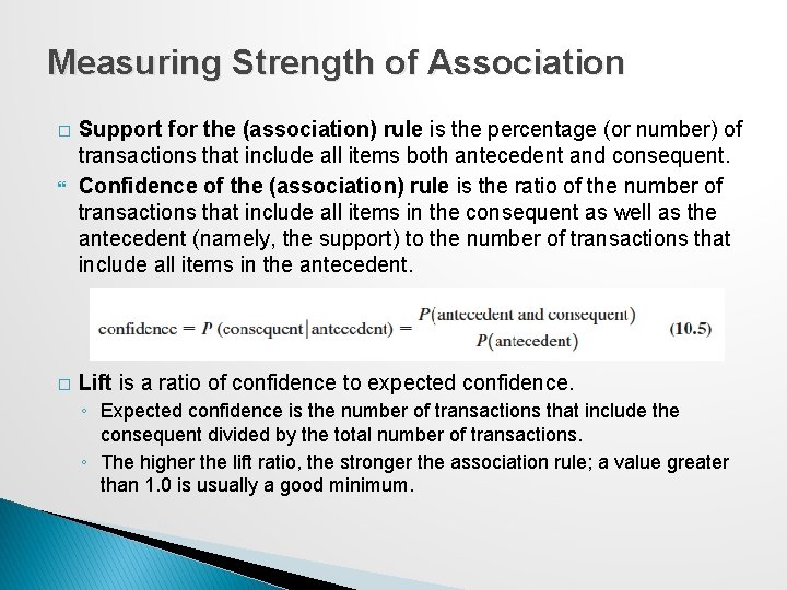
Measuring Strength of Association � � Support for the (association) rule is the percentage (or number) of transactions that include all items both antecedent and consequent. Confidence of the (association) rule is the ratio of the number of transactions that include all items in the consequent as well as the antecedent (namely, the support) to the number of transactions that include all items in the antecedent. Lift is a ratio of confidence to expected confidence. ◦ Expected confidence is the number of transactions that include the consequent divided by the total number of transactions. ◦ The higher the lift ratio, the stronger the association rule; a value greater than 1. 0 is usually a good minimum.

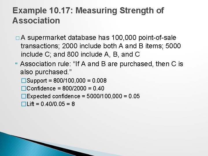
Example 10. 17: Measuring Strength of Association �A supermarket database has 100, 000 point-of-sale transactions; 2000 include both A and B items; 5000 include C; and 800 include A, B, and C Association rule: “If A and B are purchased, then C is also purchased. ” �Support = 800/100, 000 = 0. 008 �Confidence = 800/2000 = 0. 40 �Expected confidence = 5000/100, 000 = 0. 05 �Lift = 0. 40/0. 05 = 8

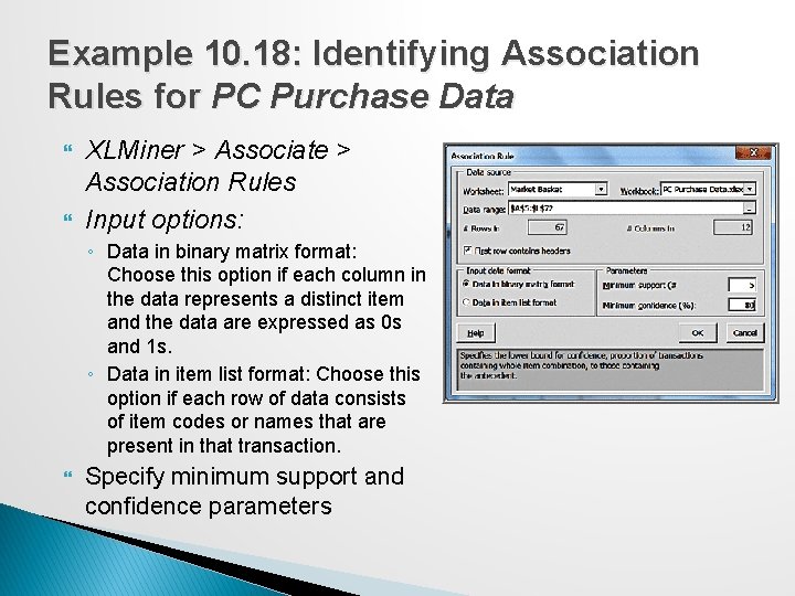
Example 10. 18: Identifying Association Rules for PC Purchase Data XLMiner > Associate > Association Rules Input options: ◦ Data in binary matrix format: Choose this option if each column in the data represents a distinct item and the data are expressed as 0 s and 1 s. ◦ Data in item list format: Choose this option if each row of data consists of item codes or names that are present in that transaction. Specify minimum support and confidence parameters

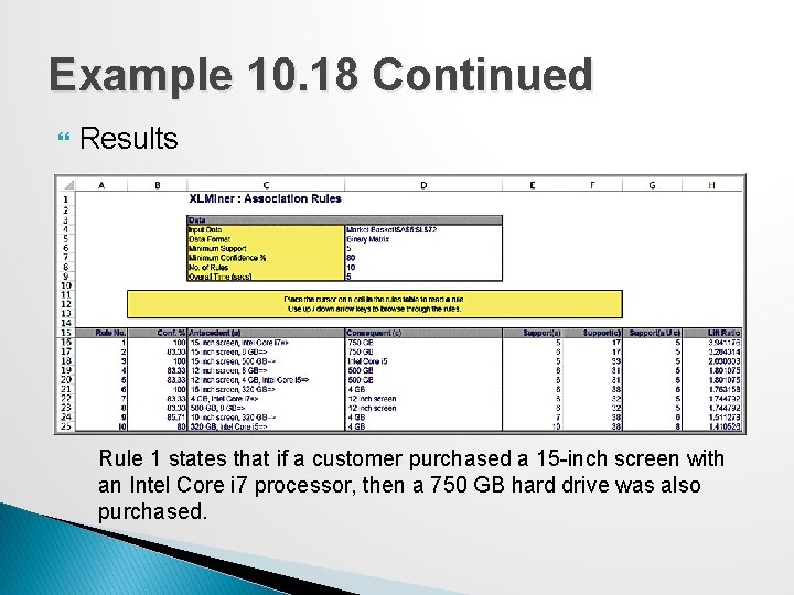
Example 10. 18 Continued Results Rule 1 states that if a customer purchased a 15 -inch screen with an Intel Core i 7 processor, then a 750 GB hard drive was also purchased.

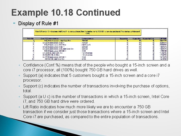
Example 10. 18 Continued Display of Rule #1 ◦ Confidence (Conf. %) means that of the people who bought a 15 -inch screen and a core i 7 processor, all (100%) bought 750 GB hard drives as well. ◦ Support (a) indicates that 5 customers bought a 15 -inch screen and a core i 7 processor. ◦ Support (c) indicates the number of transactions involving the purchase of options, total. ◦ Support (a U c) is the number of transactions in which a 15 -inch screen, Intel Core i 7, and 750 GB hard drive were ordered. ◦ Lift Ratio indicates how much more likely we are to encounter a 750 GB transaction if we consider just those transactions where a 15 -inch screen and Intel Core i 7 are purchased, as compared to the entire population of transactions.

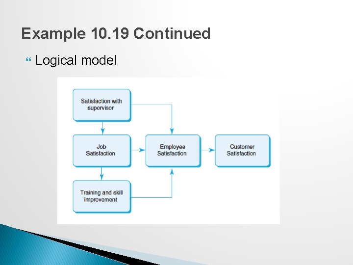
Cause-and-Effect Modeling � Correlation analysis can help us develop causeand-effect models that relate lagging and leading measures. �Lagging measures tell us what has happened and are often external business results such as profit, market share, or customer satisfaction. �Leading measures predict what will happen and are usually internal metrics such as employee satisfaction, productivity, and turnover.

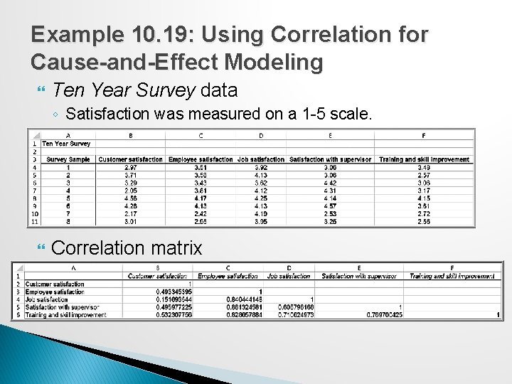
Example 10. 19: Using Correlation for Cause-and-Effect Modeling Ten Year Survey data ◦ Satisfaction was measured on a 1 -5 scale. Correlation matrix

Example 10. 19 Continued Logical model