Chapter 10 Gamma Decay Introduction Energetics of Decay

Chapter 10 Gamma Decay ● ◎ ● ◎ Introduction Energetics of γ Decay Constant for γ Decay Classical Electromagnetic Radiation Quantum Description of Electromagnetic Radiation Internal Conversion

§ 10 -1 Introduction 1. Most αandβdecays, leave the final nucleus in an excited state. Theses excited states decay rapidly to the ground state through the emission of one or moreγrays, which are photons of electromagnetic radiation. 2. Gamma rays have energy difference between the range of 0. 1 to 10 Me. V. 3. The detail and richness of out knowledge of nuclear spectroscopy depends on what we know of the excited states, and so studies of γ−ray emission have become the standard technique of nuclear spectroscopy. 4. Gamma rays are relatively easy to observe (negligible absorption and scattering in air) and their energies can be measured with high accuracy which allows good quality determination of energies on nuclear excited states. 5. Spins and parities of nuclear excited states can be deduced by properties of γdecays.

γ-ray emitting transitions 1. In this figure the vertical distance between two levels is the energy difference and the level X having the higher energy, is drawn above the one, Y, having the lower energy. 2. A transition from X to Y normally involves the emission of a photon, the energy difference going into photon energy and energy of the recoil nucleus. 3. Photon energies involved in this type of transition usually are of about 10 ke. V up to 3 or 4 Me. V and are all referred as γ-rays. 4. γ-rays are emitted when the nucleus makes a transition from an excited state to a state of lower energy.

The best way to study the existence of the heaviest elements, nucleosynthesis in exploding stars, and other phenomena peculiar to the atomic nucleus is to create customized nuclei in an accelerator like Berkeley Lab's 88 -Inch Cyclotron, then capture and analyze the gamma rays these nuclei emit when they disintegrate. The Lab's Nuclear Science Division (NSD) has been a leader in building highresolution gamma-ray detectors and was the original home of the Gammasphere, the world's most sensitive. Now NSD is leading a multi-institutional collaboration to build Gammasphere's successor, the proposed Gamma-Ray Energy Tracking Array, or GRETA. http: //www. lbl. gov/Science-Articles/Archive/sabl/2007/Feb/GRETINA. html

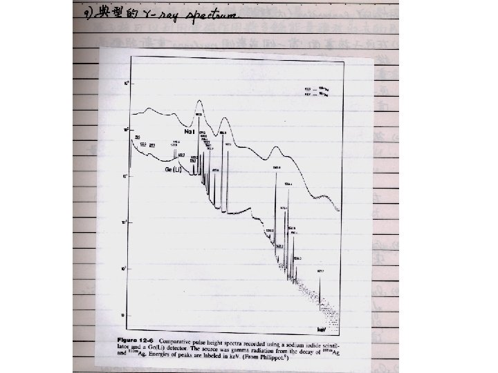
Energy spectrum observed through γ-ray emitting transitions γ-ray spectrum of 257 No Quantum states in 257 No and 253 Fm

Energy resolutions of the αparticles are not as good as γrays. Intensity against alpha energy for four isotopes, note that the line width is wide and some of the fine details can not be seen. This is for liquid scintillation counting where random effects cause a variation in the number of visible photons generated per alpha decay

§ 10 -2 Energetics of γDecay Consider the decay of a nucleus of mass M at rest, from an initial excited state Ei to a final state Ef : conservation of total energy conservation of linear momentum Define energy difference between two levels And using the relativistic relationship The energy difference ΔE is The equation (3) has the solution (1) (2) (3) (4)

(4) The energy difference ΔE are typically of the order of Me. V, while the rest energies Mc 2 are of order A × 103 Me. V, where A is the mass number. Thus ΔE << Mc 2 and to a precision of the order of 10 -4 to 10 -5 we keep only the first three terms in the expansion of the square root: (5) The actual γ-ray energy is thus diminished somewhat from the maximum available decay energy ΔE. This recoil correction to the energy is generally negligible, amounting to a 10 -5 correction that is usually far smaller than the experimental uncertainty with which we can measure energies.

§ 10 -3 Decay Constant for γDecay In atomic physics the half life of an electromagnetically excited state is of the order 10 -8 second. In nuclear physics it can range from 10 -16 second to 100 years. Time scale of this sort can be roughly estimated through a semi-classical consideration. A burst of gamma rays from space. http: //spaceknowledge. net/wp-content/gallery/nebulea/phot-40 f-99 -normal. jpg

Consider a point charge with an elementary unit of charge e. This point charge is accelerated with an acceleration. The radiation power expressed in cgs unit system is: with (6) If a point charge is in a simple harmonic motion then and where R is the radius of an atom or a nucleus. In such case the acceleration The average radiation power is thus (7) This is a classical description of the average radiation power from a point charge in a simple harmonic motion.

Quantum-mechanically an electromagnetically unstable system would emit a photon in every mean time interval τ, the average radiation power then is (8) If we define a decay constant Combining equations (7) and (8): Since the photon energy We may get the following relation: (9)

(9) The decay constant is proportional to the square of the radius of the atom (or nucleus) under study and is proportional to the cube of the photon energy Eγ. (1). In an atom take Eγ=1 e. V, R = 10 -8 cm = 1 Å (10) (2). In a nucleus take Eγ=1 Me. V, R = 5 × 10 -13 cm = 5 F (11)

Basically we are able to obtain a reasonable estimation for the half life of an electromagnetically unstable nucleus. It is of the order 10 -16 second. In reality the half life of all unstable nuclei ranges from 10 -16 second to 100 years. There are obviously some important factors which have been left out in the oversimplified semi-classical picture. We need to explore further on this topic. Electromagnetic radiation can be treated either as a classical wave phenomenon or else as a quantum phenomenon. For analyzing radiations from individual atoms and nuclei the quantum description is most appropriate, but we can more easily understand the quantum calculations of electromagnetic radiation if we first review the classical description.

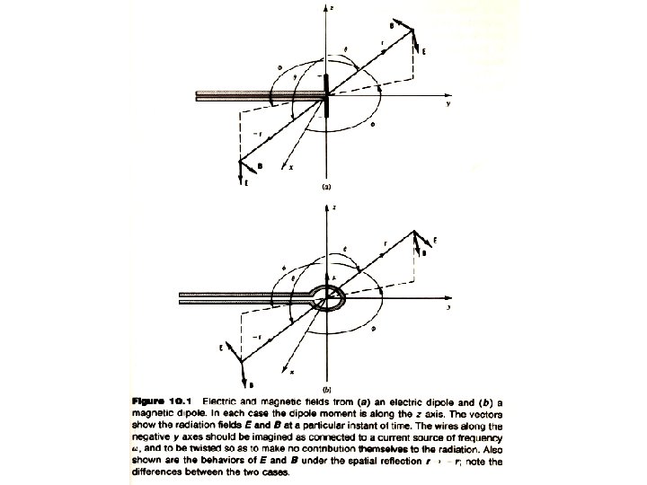
§ 10 - 4 Classical Electromagnetic Radiation Static distributions of charges and currents give static electric and magnetic fields. These fields can be analyzed in terms of the multipole moments of the charge (or current) distribution. Multipole moments ― dipole moment, quadrupole moment, etc ― give characteristic fields, and we can conveniently study the dipole field, quadrupole field and so on. Electric dipole radiation Electric quadrupole radiation

Electric Dipole Radiation Put an oscillating dipole along the z direction (12) with Then the Poynting vector is: Within a period the average quantity is The total average radiation power is (13)

Magnetic Dipole Radiation Build up an current such that its magnetic dipole is along the z direction (14) with Then the Poynting vector is: Within a period the average quantity is The total average radiation power is (15)

For electric dipole radiation For magnetic dipole radiation Same radiation patterns

There are three characteristics of the dipole radiation field that are important for us to consider: 1. The power radiated into a small element of area, in a direction at an angle θ with respect to the z axis, varies as sin 2θ. This characteristic sin 2θdependence of dipole radiation must also be a characteristic result of the quantum calculation as well. Radiations caused by higher order multipoles have different power angular distributions. 2. Electric and magnetic dipole fields have opposite parity. Under the parity transformation, the magnetic field of the electric dipole changes sign: B(r) = -B(-r) but for the magnetic dipole B(r) = B(-r). 3. The average radiated power is and for electric dipoles for magnetic dipoles Here p 0 and m 0 are the amplitudes of the time varying dipole moments.

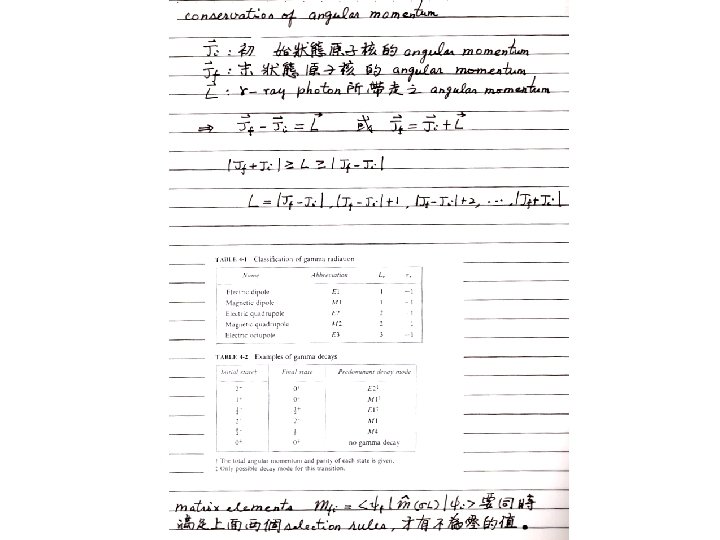
Without entering into a detailed discussion of electromagnetic theory, the properties of dipole radiation can be extended to multipole radiation in general. 1. The angular distribution of the 2 L-pole radiation, relative to a properly chosen direction, is governed by the Legendre polynomial P 2 L(cosθ). The most common cases are dipole quadrupole 2. The parity of the radiation field is Here M is for magnetic and E is for electric. 3. The radiated power is, using σ= E or M to represent electric and magnetic radiation (16) where m(σL) is the amplitude of the (time varying) electric or magnetic multipole moment.

§ 10 - 5 Quantum Description of Electromagnetic Radiation To carry the classical theory into the quantum domain, we must quantize the sources of the radiation field, the classical multipole moments. In equation (16) it is necessary to replace the multipole moments by appropriate multipole operators that change the nucleus from its initial state ψi to the final state ψf. (17) This integral is carried out over the volume of the nucleus. is the multipole operator which can be obtained by quantizing the radiation field. If we regard the equation (16) as the energy radiated per unit time in the form of then the probability per unit time for photons, each of which has energy photon emission is (18)

(18) The expression for the decay constant can be carried no further until we evaluate the matrix element mfi(σL), which requires knowledge of the initial and final wave functions. We can simplify the calculation by the assumption that the transition is due to a single proton that changes from one shell-model state to another. By so doing the EL transition probability is estimated to be (19) With R = R 0 A 1/3, we can make the following estimates for some of the lower multipole orders.

EL transition probability (19) where λ is in s-1 and E in Me. V (20)

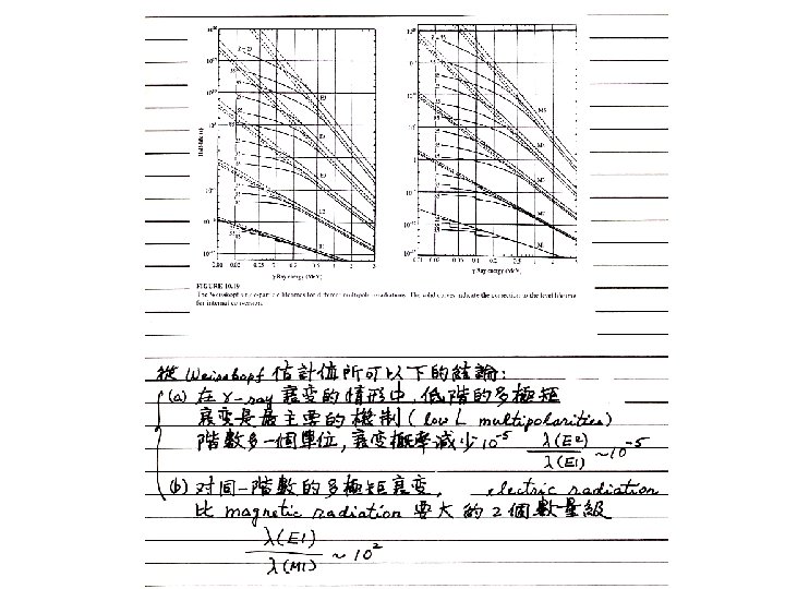
The result for the ML transition probability is (21) It is customary to replace the factor [μp 1/(L+1)]2 by 10, which gives the following estimates for the lower multipole orders: (22) These estimates for the transition rates are known as Weisskopf estimates and are not meant to be true theoretical calculations. They only provide us with reasonable relative comparisons of the transition rates.

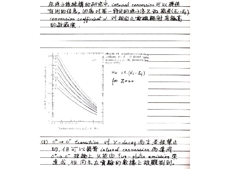
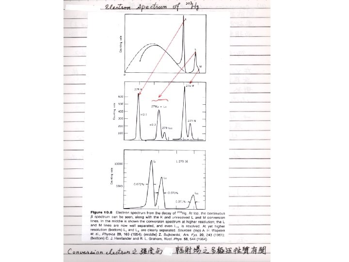
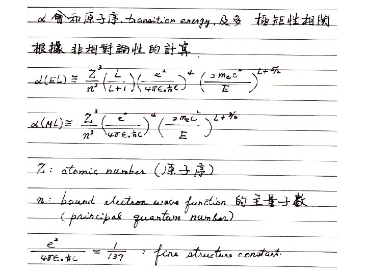
§ 10 - 6 Internal Conversion

An artist's conception of the blazar BL Lacertae at it spurts out jets of charged particles accelerated by corkscrew magnetic field lines. Credit: Marscher et al. , Wolfgang Steffen, Cosmovision, NRAO/AUI/NSF