Chapter 10 Experimental Design and Analysis of Variance

Chapter 10 Experimental Design and Analysis of Variance Mc. Graw-Hill/Irwin Copyright © 2007 by The Mc. Graw-Hill Companies, Inc. All rights reserved.

Experimental Design and Analysis of Variance 10. 1 10. 2 10. 3 10. 4 Basic Concepts of Experimental Design One-Way Analysis of Variance The Randomized Block Design Two-Way Analysis of Variance 2

Experimental Design #1 • Up until now, have considered only two ways of collecting and comparing data: • Use independent random samples • Use paired (or matched) samples • Often data is collected as the result of an experiment • To systematically study how one or more factors (variables) influence the variable that is being studied 3

Experimental Design #2 • In an experiment, there is strict control over the factors contributing to the experiment • The values or levels of the factors are called treatments • For example, in testing a medical drug, the experimenters decide which participants in the test get the drug and which ones get the placebo, instead of leaving the choice to the subjects • The object is to compare and estimate the effects of different treatments on the response variable 4

Experimental Design #3 • The different treatments are assigned to objects (the test subjects) called experimental units • When a treatment is applied to more than one experimental unit, the treatment is being “replicated” • A designed experiment is an experiment where the analyst controls which treatments used and how they are applied to the experimental units 5

Experimental Design #4 • In a completely randomized experimental design, independent random samples are assigned to each of the treatments • For example, suppose three experimental units are to be assigned to five treatments • For completely randomized experimental design randomly pick three experimental units for one treatment, randomly pick three different experimental units from those remaining for the next treatment, and so on 6

Experimental Design #5 • Once the experimental units are assigned and the experiment is performed, a value of the response variable is observed for each experimental unit • Obtain a sample of values for the response variable for each treatment 7

Experimental Design #6 • In a completely randomized experimental design, it is presumed that each sample is a random sample from the population of all possible values of the response variable • That could possibly be observed when using the specific treatment • The samples are independent of each other • Reasonable because the completely randomized design ensures that each sample results from different measurements being taken on different experimental units • Can also say that an independent samples experiment is being performed 8

One-Way Analysis of Variance • Want to study the effects of all p treatments on a response variable • For each treatment, find the mean and standard deviation of all possible values of the response variable when using that treatment • For treatment i, find treatment mean mi • One-way analysis of variance estimates and compares the effects of the different treatments on the response variable • By estimating and comparing the treatment means m 1, m 2, …, mp • One-way analysis of variance, or one-way ANOVA 9

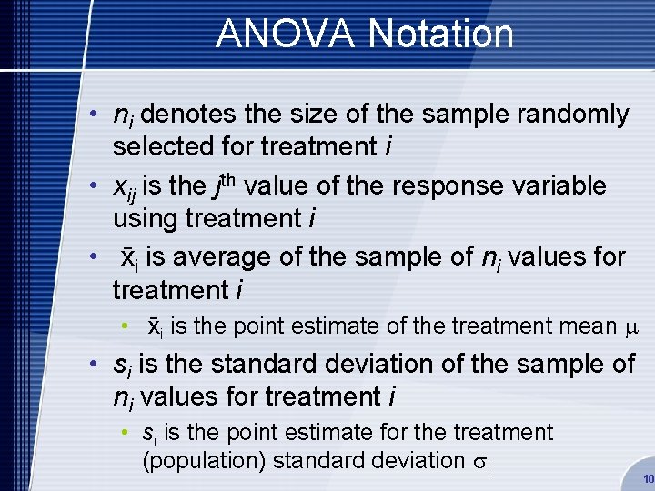
ANOVA Notation • ni denotes the size of the sample randomly selected for treatment i • xij is the jth value of the response variable using treatment i • xi is average of the sample of ni values for treatment i • xi is the point estimate of the treatment mean mi • si is the standard deviation of the sample of ni values for treatment i • si is the point estimate for the treatment (population) standard deviation si 10

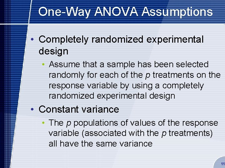
One-Way ANOVA Assumptions • Completely randomized experimental design • Assume that a sample has been selected randomly for each of the p treatments on the response variable by using a completely randomized experimental design • Constant variance • The p populations of values of the response variable (associated with the p treatments) all have the same variance 11

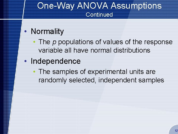
One-Way ANOVA Assumptions Continued • Normality • The p populations of values of the response variable all have normal distributions • Independence • The samples of experimental units are randomly selected, independent samples 12

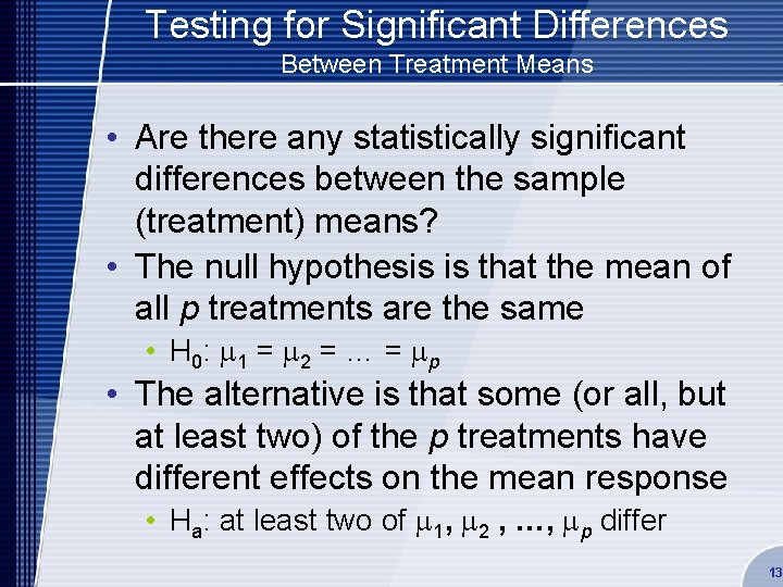
Testing for Significant Differences Between Treatment Means • Are there any statistically significant differences between the sample (treatment) means? • The null hypothesis is that the mean of all p treatments are the same • H 0: m 1 = m 2 = … = m p • The alternative is that some (or all, but at least two) of the p treatments have different effects on the mean response • Ha: at least two of m 1, m 2 , …, mp differ 13

Testing for Significant Differences Between Treatment Means Continued • Compare the between-treatment variability to the within-treatment variability • Between-treatment variability is the variability of the sample means, sample to sample • Within-treatment variability is the variability of the treatments (that is, the values) within each sample 14

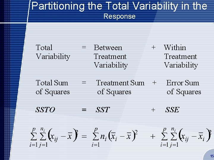
Partitioning the Total Variability in the Response Total Variability = Between Treatment Variability + Within Treatment Variability Total Sum of Squares = Treatment Sum + of Squares SSTO = SST + Error Sum of Squares SSE 15

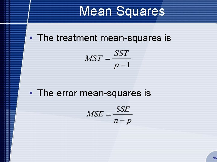
Mean Squares • The treatment mean-squares is • The error mean-squares is 16

F Test for Difference Between Treatment Means • Suppose that we want to compare p treatment means • The null hypothesis is that all treatment means are the same: • H 0: m 1 = m 2 = … = m p • The alternative hypothesis is that they are not all the same: • Ha: at least two of m 1, m 2 , …, mp differ 17

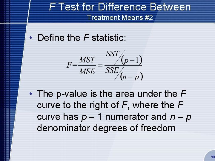
F Test for Difference Between Treatment Means #2 • Define the F statistic: • The p-value is the area under the F curve to the right of F, where the F curve has p – 1 numerator and n – p denominator degrees of freedom 18

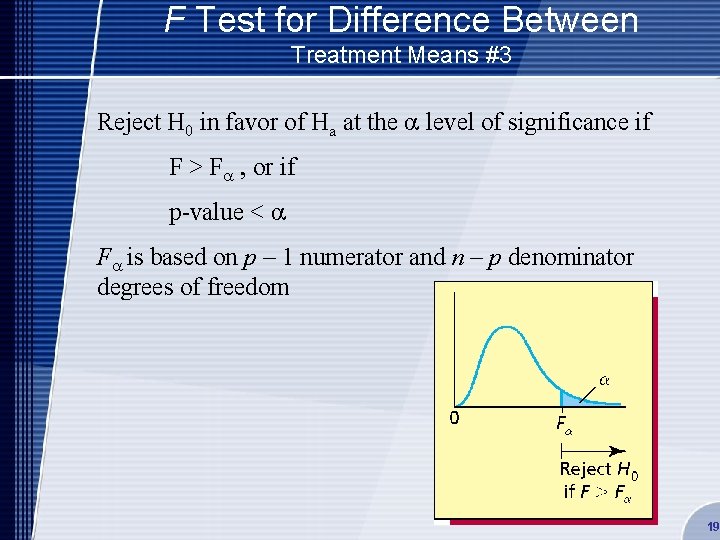
F Test for Difference Between Treatment Means #3 Reject H 0 in favor of Ha at the level of significance if F > F , or if p-value < F is based on p – 1 numerator and n – p denominator degrees of freedom 19

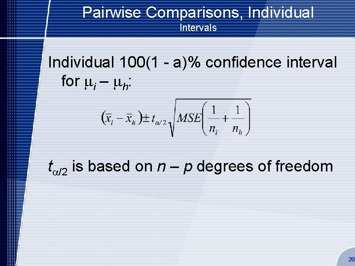
Pairwise Comparisons, Individual Intervals Individual 100(1 - a)% confidence interval for mi – mh: t /2 is based on n – p degrees of freedom 20

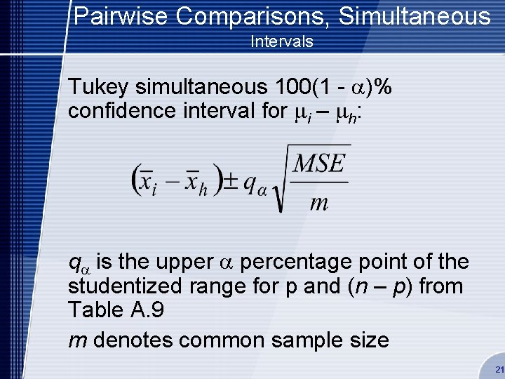
Pairwise Comparisons, Simultaneous Intervals Tukey simultaneous 100(1 - )% confidence interval for mi – mh: q is the upper percentage point of the studentized range for p and (n – p) from Table A. 9 m denotes common sample size 21

The Randomized Block Design • A randomized block design compares p treatments (for example, production methods) on each of b blocks (or experimental units or sets of units; for example, machine operators) • Each block is used exactly once to measure the effect of each and every treatment • The order in which each treatment is assigned to a block should be random • A generalization of the paired difference design, this design controls for variability in experimental units by comparing each treatment on the same (not independent) experimental units • Differences in the treatments are not hidden by differences in the experimental units (the blocks) 22

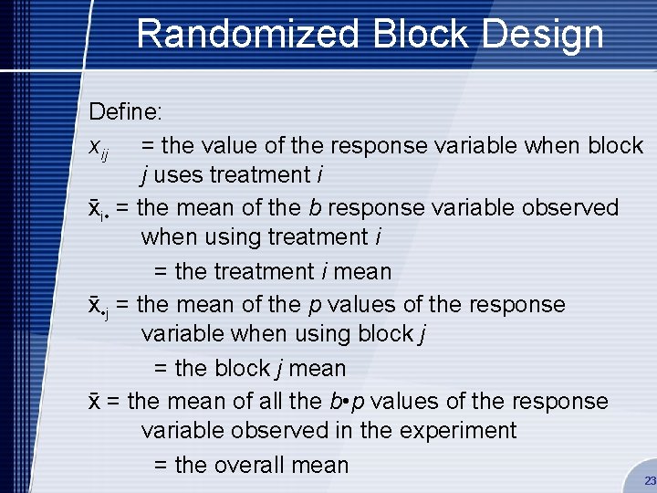
Randomized Block Design Define: xij = the value of the response variable when block j uses treatment i xi • = the mean of the b response variable observed when using treatment i = the treatment i mean x • j = the mean of the p values of the response variable when using block j = the block j mean x = the mean of all the b • p values of the response variable observed in the experiment = the overall mean 23

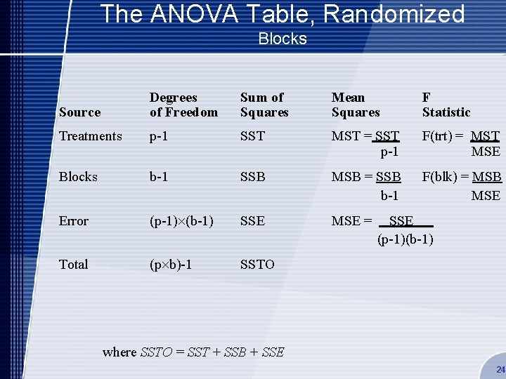
The ANOVA Table, Randomized Blocks Source Degrees of Freedom Sum of Squares Mean Squares F Statistic Treatments p-1 SST MST = SST p-1 F(trt) = MST MSE Blocks b-1 SSB MSB = SSB b-1 F(blk) = MSB MSE Error (p-1) (b-1) SSE MSE = Total (p b)-1 SSTO SSE (p-1)(b-1) where SSTO = SST + SSB + SSE 24

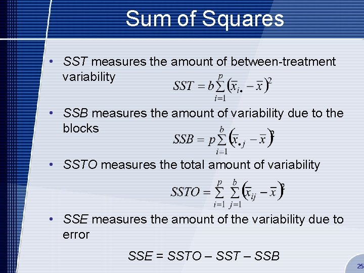
Sum of Squares • SST measures the amount of between-treatment variability • SSB measures the amount of variability due to the blocks • SSTO measures the total amount of variability • SSE measures the amount of the variability due to error SSE = SSTO – SST – SSB 25

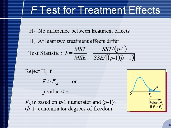
F Test for Treatment Effects H 0: No difference between treatment effects Ha: At least two treatment effects differ Reject H 0 if F > F or p-value < F is based on p-1 numerator and (p-1) (b-1) denominator degrees of freedom 26

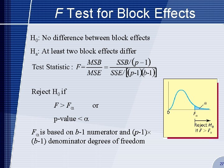
F Test for Block Effects H 0: No difference between block effects Ha: At least two block effects differ Reject H 0 if F > F or p-value < F is based on b-1 numerator and (p-1) (b-1) denominator degrees of freedom 27

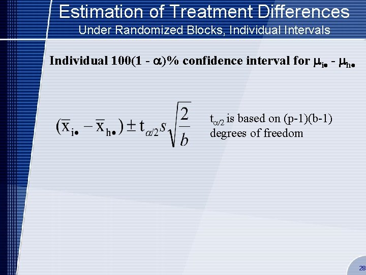
Estimation of Treatment Differences Under Randomized Blocks, Individual Intervals Individual 100(1 - a)% confidence interval for mi - mh t /2 is based on (p-1)(b-1) degrees of freedom 28

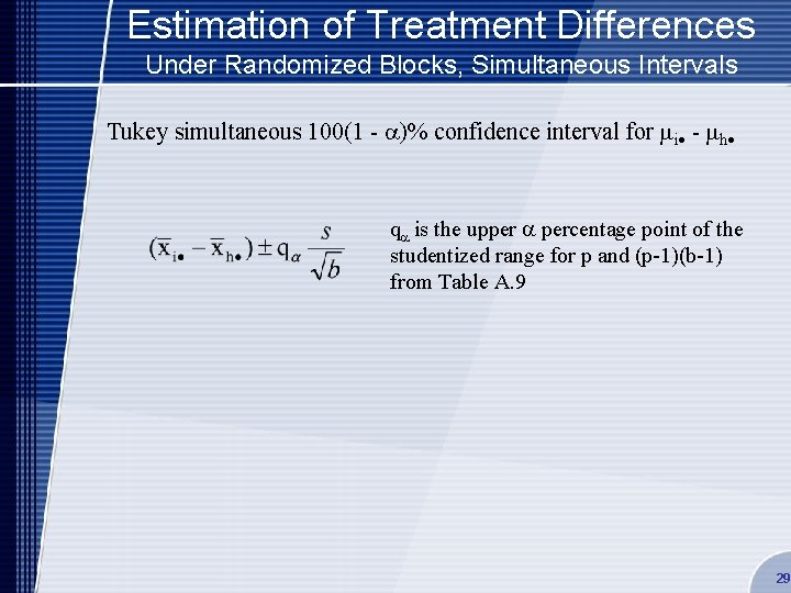
Estimation of Treatment Differences Under Randomized Blocks, Simultaneous Intervals Tukey simultaneous 100(1 - )% confidence interval for mi - mh q is the upper percentage point of the studentized range for p and (p-1)(b-1) from Table A. 9 29

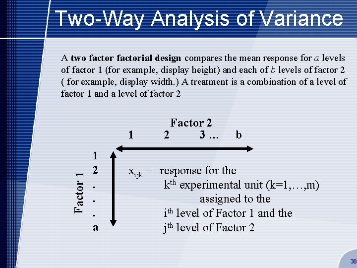
Two-Way Analysis of Variance A two factorial design compares the mean response for a levels of factor 1 (for example, display height) and each of b levels of factor 2 ( for example, display width. ) A treatment is a combination of a level of factor 1 and a level of factor 2 Factor 1 1 1 2. . . a Factor 2 2 3… b xijk = response for the kth experimental unit (k=1, …, m) assigned to the ith level of Factor 1 and the jth level of Factor 2 30

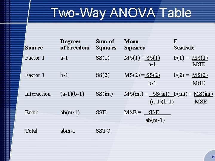
Two-Way ANOVA Table Source Degrees of Freedom Sum of Squares Mean Squares F Statistic Factor 1 a-1 SS(1) MS(1) = SS(1) a-1 F(1) = MS(1) MSE Factor 1 b-1 SS(2) MS(2) = SS(2) b-1 F(2) = MS(2) MSE Interaction (a-1)(b-1) SS(int) MS(int) = SS(int) F(int) = MS(int) (a-1)(b-1) MSE Error ab(m-1) SSE MSE = Total abm-1 SSTO SSE ab(m-1) 31

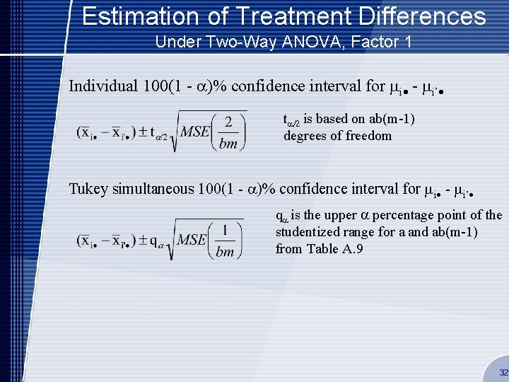
Estimation of Treatment Differences Under Two-Way ANOVA, Factor 1 Individual 100(1 - )% confidence interval for mi - mi’ t /2 is based on ab(m-1) degrees of freedom Tukey simultaneous 100(1 - )% confidence interval for mi - mi’ q is the upper percentage point of the studentized range for a and ab(m-1) from Table A. 9 32

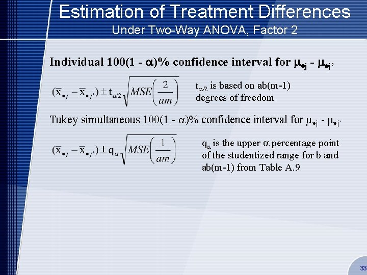
Estimation of Treatment Differences Under Two-Way ANOVA, Factor 2 Individual 100(1 - a)% confidence interval for m j - m j’ t /2 is based on ab(m-1) degrees of freedom Tukey simultaneous 100(1 - )% confidence interval for m j - m j’ q is the upper percentage point of the studentized range for b and ab(m-1) from Table A. 9 33