Chapter 10 DiscreteTime Linear TimeInvariant Systems Sections 10

Chapter 10 Discrete-Time Linear Time-Invariant Systems Sections 10. 1 -10 -3

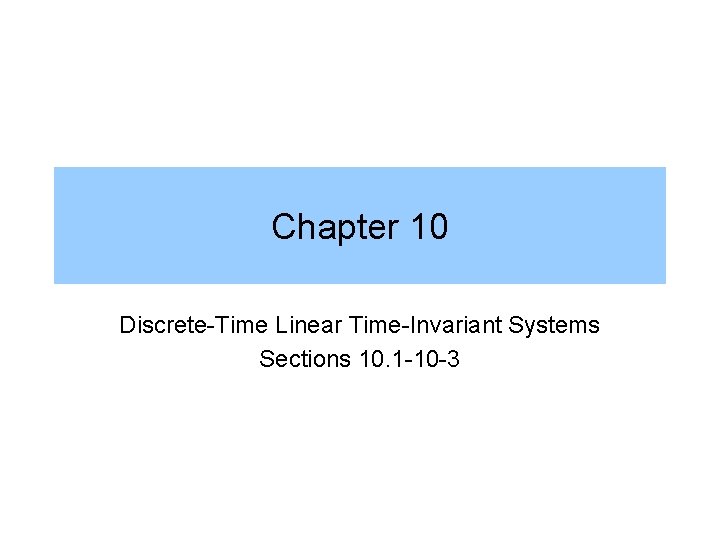
Representation of Discrete-Time Signals • We assume Discrete-Time LTI systems • The signal X[n] can be represented using unit sample function or unit impulse function: d[n] • Remember: • Notations: notes

Representation of Discrete-Time Signals - Example

Convolution for Discrete-Time Systems • LTI system response can be described using: d[n] • For time-invariant: d[n-k] h[n-k] • For a linear system: x[k]d[n-k] x[k]h[n-k] • Remember: • Thus, for LTI: • We call this the convolution sum • Remember: System h[n] Impulse Response of a System

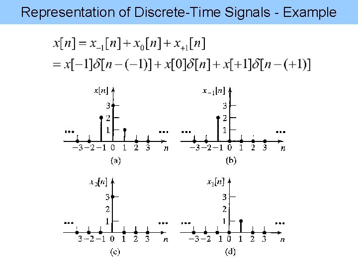
Convolution for Discrete-Important Properties • By definition • Remember (due to time-invariance property): • Multiplication

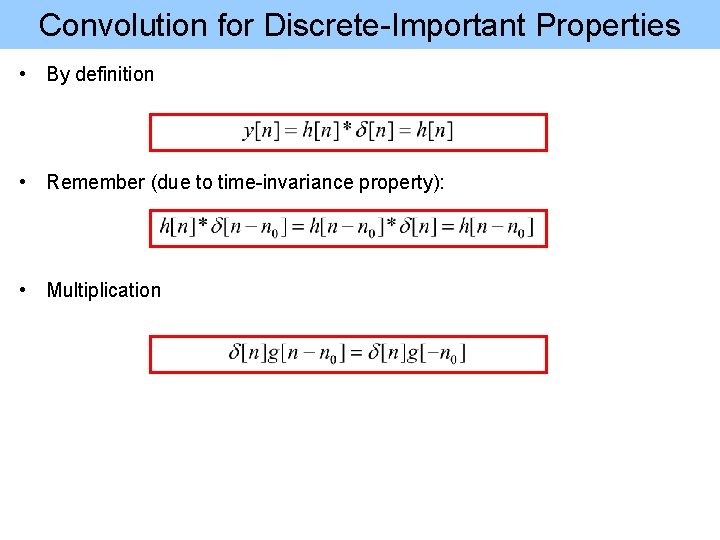
Properties of Convolution • Commutative • Associative • Distributive

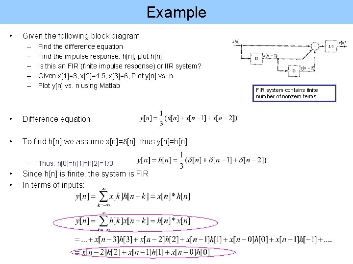
Example • Given the following block diagram – – – Find the difference equation Find the impulse response: h[n]; plot h[n] Is this an FIR (finite impulse response) or IIR system? Given x[1]=3, x[2]=4. 5, x[3]=6, Plot y[n] vs. n using Matlab • Difference equation • To find h[n] we assume x[n]=d[n], thus y[n]=h[n] – Thus: h[0]=h[1]=h[2]=1/3 • • Since h[n] is finite, the system is FIR In terms of inputs: Figure 10. 3 FIR system contains finite number of nonzero terms

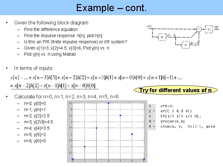
Example – cont. • Given the following block diagram – – – • Find the difference equation Find the impulse response: h[n]; plot h[n] Is this an FIR (finite impulse response) or IIR system? Given x[1]=3, x[2]=4. 5, x[3]=6, Plot y[n] vs. n using Matlab Figure 10. 3 In terms of inputs: Try for different values of n • Calculate for n=0, n=1, n=2, n=3, n=4, n=5, n=6 – – – – n=0; y[0]=0 n=1; y[n]=1 n=2; y[2]=2. 5 n=3; y[23]=4. 5 n=4; y[4]=3. 5 n=5; y[5]=2 n=6; y[6]=0

Example – cont. (Graphical Representation) X[m] h[0]=h[1]=h[2]=1/3 x[1]=3, x[2]=4. 5, x[3]=6 X[n-k]

Example • Consider the following difference equation: y[n]=ay[n-1]+x[n] – – Draw the block diagram of this system Find the impulse response: h[n] Is it a causal system? Is this an IIR or FIR system?

Example • Consider the following difference equation: y[n]=ay[n-1]+x[n]; – Draw the block diagram of this system – Find the impulse response: h[n] – Is this an IIR or FIR system? We assume x[n]=d[n] y[n]=h[n]=ah[n-1]+d[n]; y[0]=h[0]=1 y[1]=h[1]=a y[2]=h[2]=a^2 y[3]=h[3]= a^3 h[n]=a^n ; n>=0 It is IIR (unbounded) Causal system (current and past)

Example • Assume h[n]=0. 6^n*u[n] and x[n]=u[n] – Find the expression for y[n] – Plot y[n] using Matlab x[n] h[n] y[0]=1 y[1]=1. 6 …. . y(100)=2. 5 Steady State Value is 2. 5

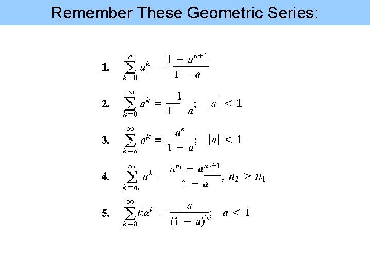
Remember These Geometric Series:

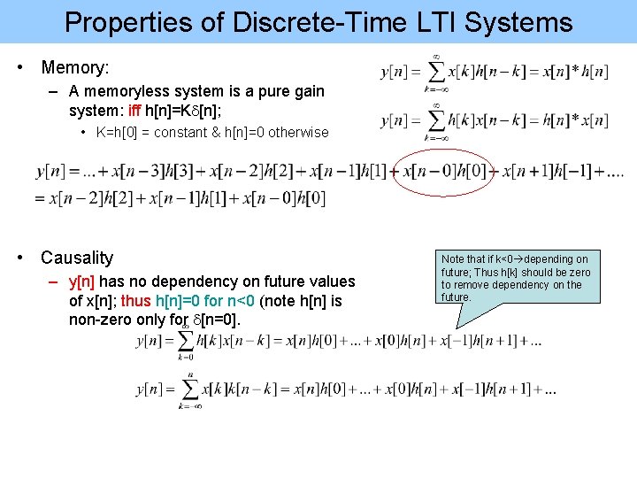
Properties of Discrete-Time LTI Systems • Memory: – A memoryless system is a pure gain system: iff h[n]=Kd[n]; • K=h[0] = constant & h[n]=0 otherwise • Causality – y[n] has no dependency on future values of x[n]; thus h[n]=0 for n<0 (note h[n] is non-zero only for d[n=0]. Note that if k<0 depending on future; Thus h[k] should be zero to remove dependency on the future.

Properties of Discrete-Time LTI Systems • Stability – BIBO: |x[n]|< M – Absolutely summable: • Invertibility: – If the input can be determined from output – It has an inverse impulse response – Invertible if there exists: hi[n]*h[n]=d[n]

Example 1 • Assume h[n]= u[n] (1/2)^n – Memoryless? – Casual system? – Stable? – Has memory (dynamic): h[n] is not Kd[n] (not pure gain); h[n] is non-zero – Is causal: h[n]=0 for n<0 – Stable: x[n] h[n] y[n]

Example 2 • Assume h[n]= u[n+1] (1/2)^n – Memoryless? – Casual system? – Stable? – Has memory (dynamic): h[n] is not Kd[n] (not pure gain) – Is NOT causal: h[n] not 0 for n<0; h[-1]=2 – Stable: x[n] h[n] y[n]

Example 3 • Assume h[n]= u[n] (2)^n – Memoryless? – Casual system? – Stable? – Has memory (dynamic): h[n] is not Kd[n] (not pure gain) – Is causal: h[n]=0 for n<0 – Not Stable: x[n] h[n] y[n]