CHAPTER 10 Dealing With Uncertainty RISK Risk and

CHAPTER 10 Dealing With Uncertainty

RISK • Risk and uncertainty are similar • Both present the problem of not knowing what future conditions will be • Risk offers estimates of probabilities for possible outcomes • Uncertainty does not provide estimates of probabilities for possible outcomes • This book treats them as interchangeable

Four Major Sources Of Uncertainty 1. Possible inaccuracy of cash-flow estimates used in the study – – How much source information is available How dependable is the source information 2. Type of business relative to the future health of the economy – Some businesses will typically be more at risk when there is a general decline in the economy 3. Type of physical plant and equipment involved 1. Some equipment have more definite lives and MV than the others (general lathe machine vs. mining equipment) 4. Length of study period – The longer the study period, the greater the level of uncertainty of a capital investment

Sensitivity Analysis • • Sensitivity – The degree to which a measure of merit (I. e. , PW, IRR, etc…) will change as a result of changes in one or more of the study factor values Sensitivity Analysis Techniques – Breakeven Analysis – Sensitivity Graph (spiderplot) – Combination of factors

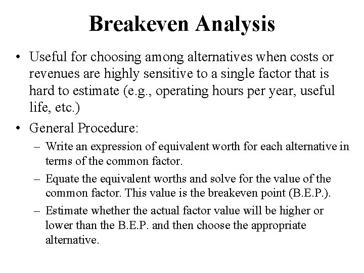
Breakeven Analysis • Useful for choosing among alternatives when costs or revenues are highly sensitive to a single factor that is hard to estimate (e. g. , operating hours per year, useful life, etc. ) • General Procedure: – Write an expression of equivalent worth for each alternative in terms of the common factor. – Equate the equivalent worths and solve for the value of the common factor. This value is the breakeven point (B. E. P. ). – Estimate whether the actual factor value will be higher or lower than the B. E. P. and then choose the appropriate alternative.

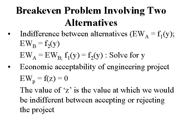
Breakeven Problem Involving Two Alternatives • • Indifference between alternatives (EWA = f 1(y); EWB = f 2(y) EWA = EWB; f 1(y) = f 2(y) : Solve for y Economic acceptability of engineering project EWp = f(z) = 0 The value of ‘z’ is the value at which we would be indifferent between accepting or rejecting the project

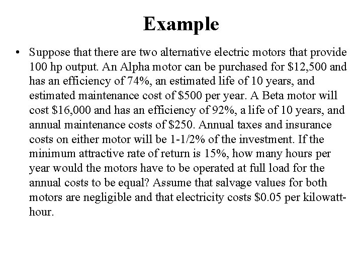
Example • Suppose that there are two alternative electric motors that provide 100 hp output. An Alpha motor can be purchased for $12, 500 and has an efficiency of 74%, an estimated life of 10 years, and estimated maintenance cost of $500 per year. A Beta motor will cost $16, 000 and has an efficiency of 92%, a life of 10 years, and annual maintenance costs of $250. Annual taxes and insurance costs on either motor will be 1 -1/2% of the investment. If the minimum attractive rate of return is 15%, how many hours per year would the motors have to be operated at full load for the annual costs to be equal? Assume that salvage values for both motors are negligible and that electricity costs $0. 05 per kilowatthour.

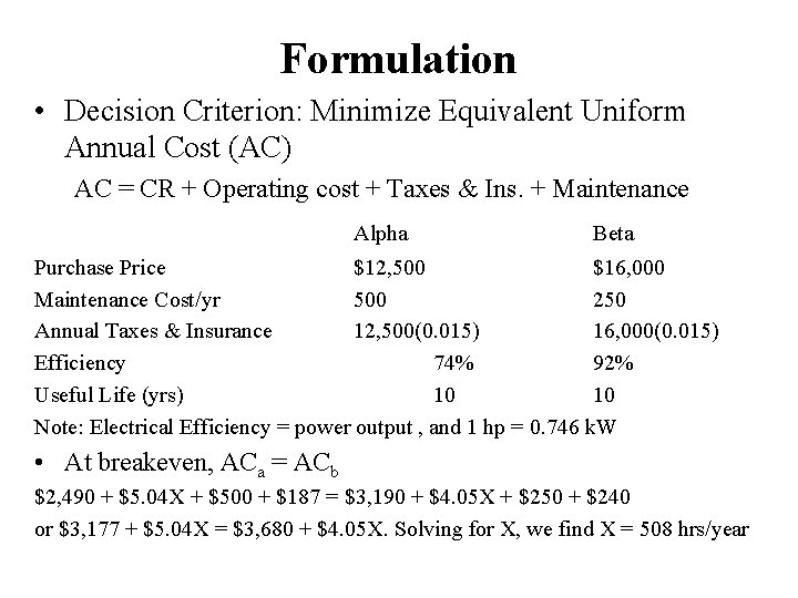
Formulation • Decision Criterion: Minimize Equivalent Uniform Annual Cost (AC) AC = CR + Operating cost + Taxes & Ins. + Maintenance Alpha Beta Purchase Price $12, 500 $16, 000 Maintenance Cost/yr 500 250 Annual Taxes & Insurance 12, 500(0. 015) 16, 000(0. 015) Efficiency 74% 92% Useful Life (yrs) 10 10 Note: Electrical Efficiency = power output , and 1 hp = 0. 746 k. W • At breakeven, ACa = ACb $2, 490 + $5. 04 X + $500 + $187 = $3, 190 + $4. 05 X + $250 + $240 or $3, 177 + $5. 04 X = $3, 680 + $4. 05 X. Solving for X, we find X = 508 hrs/year

Sensitivity Graph (Spiderplot) • Makes explicit the impact of uncertainty in the estimates of each factor of concern on the economic measure of merit – Annual revenue and expenses – Rate of return – Market (or salvage) value – Equipment Life – Capacity utilization

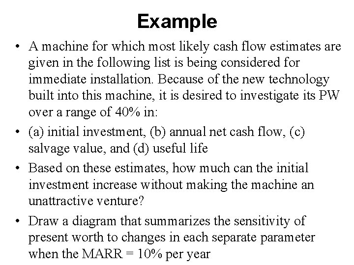
Example • A machine for which most likely cash flow estimates are given in the following list is being considered for immediate installation. Because of the new technology built into this machine, it is desired to investigate its PW over a range of 40% in: • (a) initial investment, (b) annual net cash flow, (c) salvage value, and (d) useful life • Based on these estimates, how much can the initial investment increase without making the machine an unattractive venture? • Draw a diagram that summarizes the sensitivity of present worth to changes in each separate parameter when the MARR = 10% per year

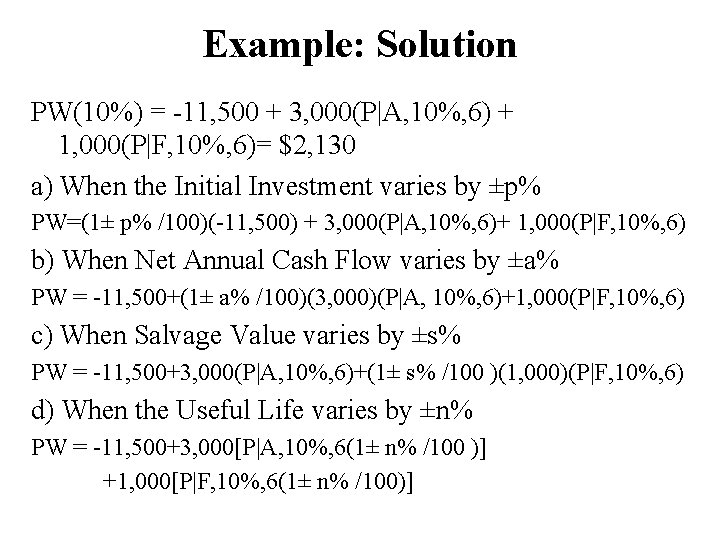
Example: Solution PW(10%) = -11, 500 + 3, 000(P|A, 10%, 6) + 1, 000(P|F, 10%, 6)= $2, 130 a) When the Initial Investment varies by ±p% PW=(1± p% /100)(-11, 500) + 3, 000(P|A, 10%, 6)+ 1, 000(P|F, 10%, 6) b) When Net Annual Cash Flow varies by ±a% PW = -11, 500+(1± a% /100)(3, 000)(P|A, 10%, 6)+1, 000(P|F, 10%, 6) c) When Salvage Value varies by ±s% PW = -11, 500+3, 000(P|A, 10%, 6)+(1± s% /100 )(1, 000)(P|F, 10%, 6) d) When the Useful Life varies by ±n% PW = -11, 500+3, 000[P|A, 10%, 6(1± n% /100 )] +1, 000[P|F, 10%, 6(1± n% /100)]

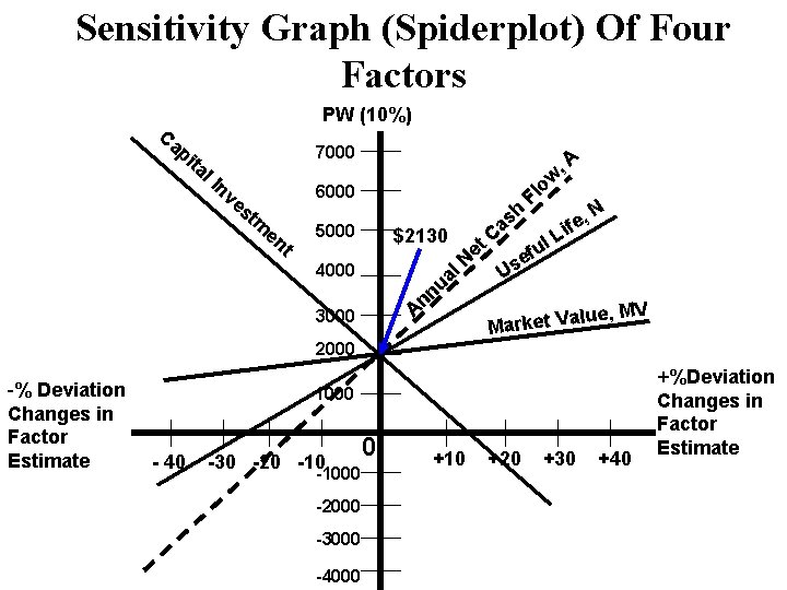
Sensitivity Graph (Spiderplot) Of Four Factors PW (10%) Ca p ita l. I 7000 nv w o Fl 6000 es t m en t , A h N , s e a if C $2130 L ul et f e l N Us a u n n A ue, MV l a V t e k r Ma 5000 4000 3000 2000 -% Deviation Changes in Factor Estimate 1000 - 40 -30 -20 -1000 -2000 -3000 -4000 0 +10 +20 +30 +40 +%Deviation Changes in Factor Estimate

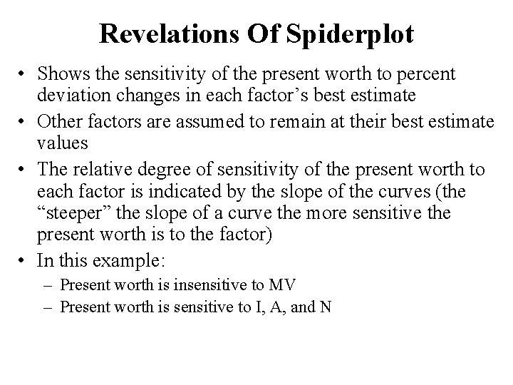
Revelations Of Spiderplot • Shows the sensitivity of the present worth to percent deviation changes in each factor’s best estimate • Other factors are assumed to remain at their best estimate values • The relative degree of sensitivity of the present worth to each factor is indicated by the slope of the curves (the “steeper” the slope of a curve the more sensitive the present worth is to the factor) • In this example: – Present worth is insensitive to MV – Present worth is sensitive to I, A, and N

Measuring Sensitivity By A Combination Of Factors • • • Develop a sensitivity graph for the project Use sensitivity graph to select most sensitive project factors. Analyze combined effects of these factors on project’s economic measure of merit

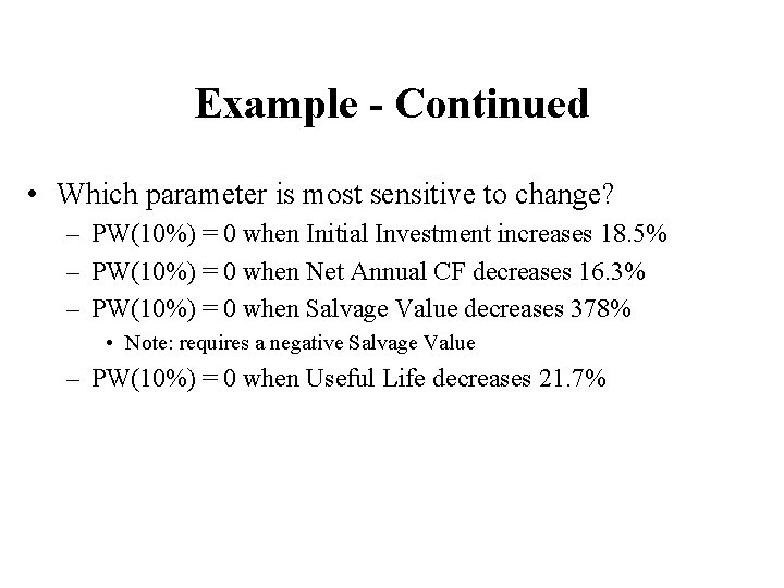
Example - Continued • Which parameter is most sensitive to change? – PW(10%) = 0 when Initial Investment increases 18. 5% – PW(10%) = 0 when Net Annual CF decreases 16. 3% – PW(10%) = 0 when Salvage Value decreases 378% • Note: requires a negative Salvage Value – PW(10%) = 0 when Useful Life decreases 21. 7%

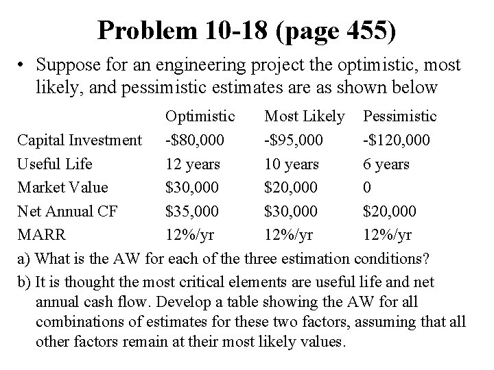
Optimistic - Pessimistic Estimates • Exploring sensitivity by estimating one or more factors in a favorable direction and in an unfavorable direction to investigate the effect on study results. – Optimistic - 95 th percentile (desirable) – Pessimistic - 5 th percentile (undesirable) • Not only do we examine the Equivalent Worth (EW) for all three estimation conditions, we examine the EW for all combinations of estimated outcomes for the key factors being estimated.

Problem 10 -18 (page 455) • Suppose for an engineering project the optimistic, most likely, and pessimistic estimates are as shown below Optimistic Most Likely Pessimistic Capital Investment -$80, 000 -$95, 000 -$120, 000 Useful Life 12 years 10 years 6 years Market Value $30, 000 $20, 000 0 Net Annual CF $35, 000 $30, 000 $20, 000 MARR 12%/yr a) What is the AW for each of the three estimation conditions? b) It is thought the most critical elements are useful life and net annual cash flow. Develop a table showing the AW for all combinations of estimates for these two factors, assuming that all other factors remain at their most likely values.

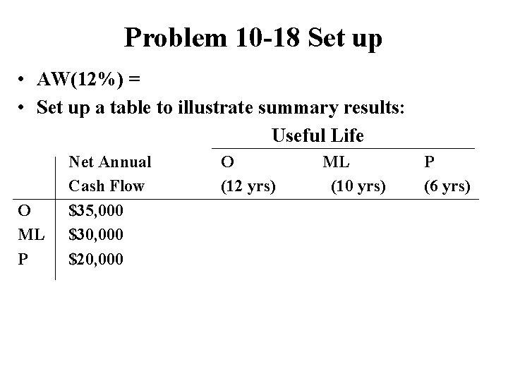
Problem 10 -18 Set up • AW(12%) = • Set up a table to illustrate summary results: Useful Life O ML P Net Annual Cash Flow $35, 000 $30, 000 $20, 000 O (12 yrs) ML (10 yrs) P (6 yrs)

Dealing with Uncertainty • Uncertainty causes factors to become random variable in engineering economy analysis • Risk-Adjusted MARR – A widely used industrial practice for including some consideration of uncertainty is to increase the MARR • Reduction of useful life – By dropping from consideration those revenues (savings) and expenses that may occur after a reduced study period, heavy emphasis is placed on rapid recovery of capital in early years of a project’s life – This method is closely related to the discounted payback technique and suffers from most of the same deficiencies