Chapter 10 CHISQUARE TESTS AND THE F DISTRIBUTION

Chapter 10 CHI-SQUARE TESTS AND THE F -DISTRIBUTION LARSON/FARBER 4 TH ED 1

Chapter Outline 10. 1 Goodness of Fit 10. 2 Independence 10. 3 Comparing Two Variances 10. 4 Analysis of Variance LARSON/FARBER 4 TH ED 2

Section 10. 1 GOODNESS OF FIT LARSON/FARBER 4 TH ED 3

Section 10. 1 Objectives Use the chi-square distribution to test whether a frequency distribution fits a claimed distribution LARSON/FARBER 4 TH ED 4

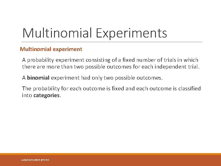
Multinomial Experiments Multinomial experiment A probability experiment consisting of a fixed number of trials in which there are more than two possible outcomes for each independent trial. A binomial experiment had only two possible outcomes. The probability for each outcome is fixed and each outcome is classified into categories. LARSON/FARBER 4 TH ED 5

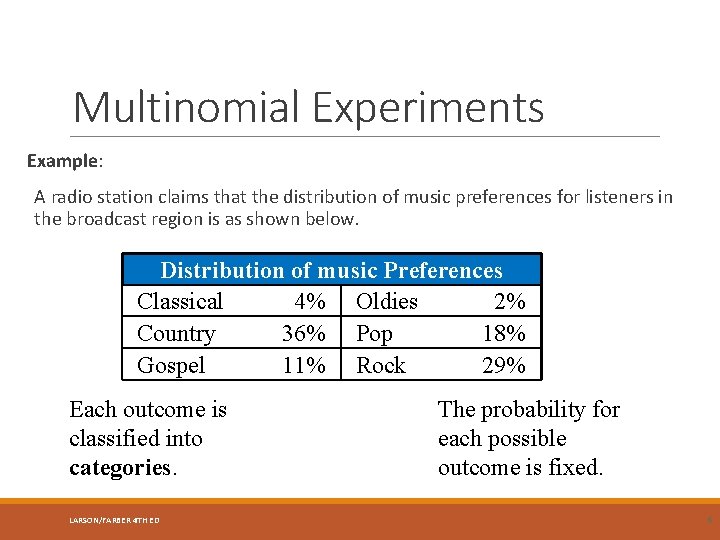
Multinomial Experiments Example: A radio station claims that the distribution of music preferences for listeners in the broadcast region is as shown below. Distribution of music Preferences Classical 4% Oldies 2% Country 36% Pop 18% Gospel 11% Rock 29% Each outcome is classified into categories. LARSON/FARBER 4 TH ED The probability for each possible outcome is fixed. 6

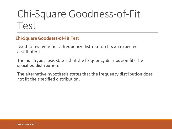
Chi-Square Goodness-of-Fit Test Used to test whether a frequency distribution fits an expected distribution. The null hypothesis states that the frequency distribution fits the specified distribution. The alternative hypothesis states that the frequency distribution does not fit the specified distribution. LARSON/FARBER 4 TH ED 7

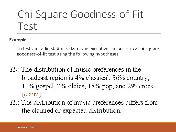
Chi-Square Goodness-of-Fit Test Example: To test the radio station’s claim, the executive can perform a chi-square goodness-of-fit test using the following hypotheses. H 0: The distribution of music preferences in the broadcast region is 4% classical, 36% country, 11% gospel, 2% oldies, 18% pop, and 29% rock. (claim) Ha: The distribution of music preferences differs from the claimed or expected distribution. LARSON/FARBER 4 TH ED 8

Chi-Square Goodness-of-Fit Test To calculate the test statistic for the chi-square goodness-of-fit test, the observed frequencies and the expected frequencies are used. The observed frequency O of a category is the frequency for the category observed in the sample data. LARSON/FARBER 4 TH ED 9

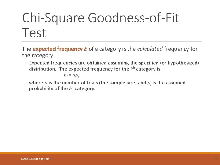
Chi-Square Goodness-of-Fit Test The expected frequency E of a category is the calculated frequency for the category. ◦ Expected frequencies are obtained assuming the specified (or hypothesized) distribution. The expected frequency for the ith category is Ei = npi where n is the number of trials (the sample size) and pi is the assumed probability of the ith category. LARSON/FARBER 4 TH ED 10

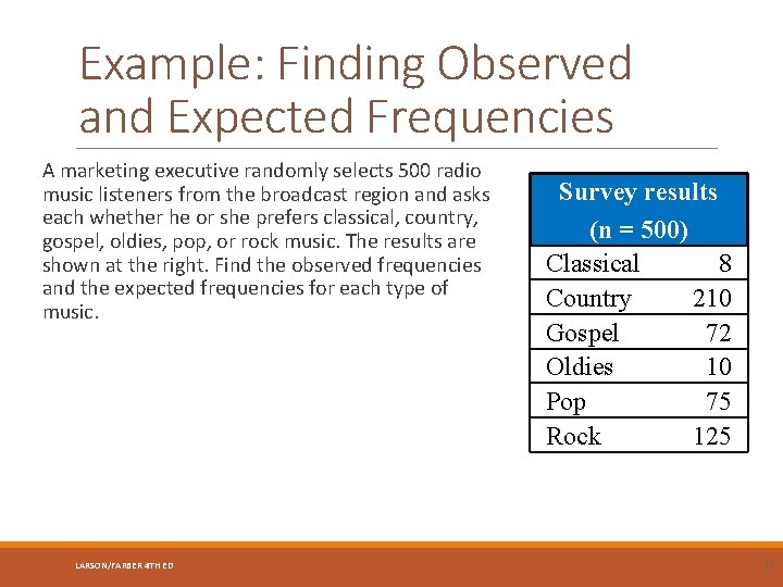
Example: Finding Observed and Expected Frequencies A marketing executive randomly selects 500 radio music listeners from the broadcast region and asks each whether he or she prefers classical, country, gospel, oldies, pop, or rock music. The results are shown at the right. Find the observed frequencies and the expected frequencies for each type of music. LARSON/FARBER 4 TH ED Survey results (n = 500) Classical 8 Country 210 Gospel 72 Oldies 10 Pop 75 Rock 125 11

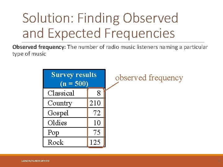
Solution: Finding Observed and Expected Frequencies Observed frequency: The number of radio music listeners naming a particular type of music Survey results (n = 500) Classical 8 Country 210 Gospel 72 Oldies 10 Pop 75 Rock 125 LARSON/FARBER 4 TH ED observed frequency 12

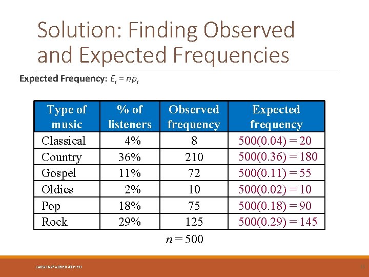
Solution: Finding Observed and Expected Frequencies Expected Frequency: Ei = npi Type of music Classical Country Gospel Oldies Pop Rock LARSON/FARBER 4 TH ED % of listeners 4% 36% 11% 2% 18% 29% Observed frequency 8 210 72 10 75 125 n = 500 Expected frequency 500(0. 04) = 20 500(0. 36) = 180 500(0. 11) = 55 500(0. 02) = 10 500(0. 18) = 90 500(0. 29) = 145 13

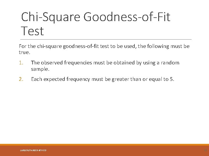
Chi-Square Goodness-of-Fit Test For the chi-square goodness-of-fit test to be used, the following must be true. 1. The observed frequencies must be obtained by using a random sample. 2. Each expected frequency must be greater than or equal to 5. LARSON/FARBER 4 TH ED 14

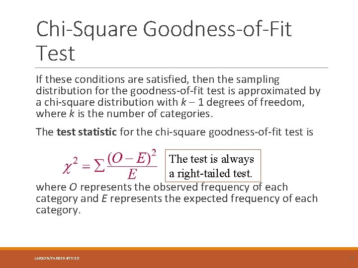
Chi-Square Goodness-of-Fit Test If these conditions are satisfied, then the sampling distribution for the goodness-of-fit test is approximated by a chi-square distribution with k – 1 degrees of freedom, where k is the number of categories. The test statistic for the chi-square goodness-of-fit test is The test is always a right-tailed test. where O represents the observed frequency of each category and E represents the expected frequency of each category. LARSON/FARBER 4 TH ED 15

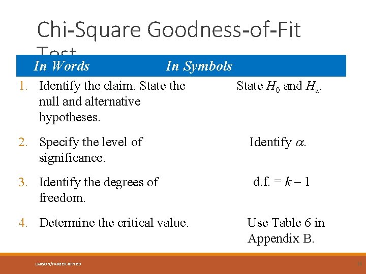
Chi-Square Goodness-of-Fit Test In Words In Symbols 1. Identify the claim. State the null and alternative hypotheses. State H 0 and Ha. 2. Specify the level of significance. Identify . 3. Identify the degrees of freedom. d. f. = k – 1 4. Determine the critical value. LARSON/FARBER 4 TH ED Use Table 6 in Appendix B. 16

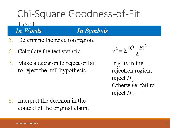
Chi-Square Goodness-of-Fit Test In Words In Symbols 5. Determine the rejection region. 6. Calculate the test statistic. 7. Make a decision to reject or fail to reject the null hypothesis. 8. Interpret the decision in the context of the original claim. LARSON/FARBER 4 TH ED If χ2 is in the rejection region, reject H 0. Otherwise, fail to reject H 0. 17

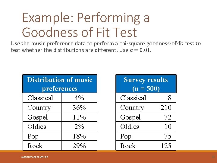
Example: Performing a Goodness of Fit Test Use the music preference data to perform a chi-square goodness-of-fit test to test whether the distributions are different. Use α = 0. 01. Distribution of music preferences Classical 4% Country 36% Gospel 11% Oldies 2% Pop 18% Rock 29% LARSON/FARBER 4 TH ED Survey results (n = 500) Classical 8 Country 210 Gospel 72 Oldies 10 Pop 75 Rock 125 18

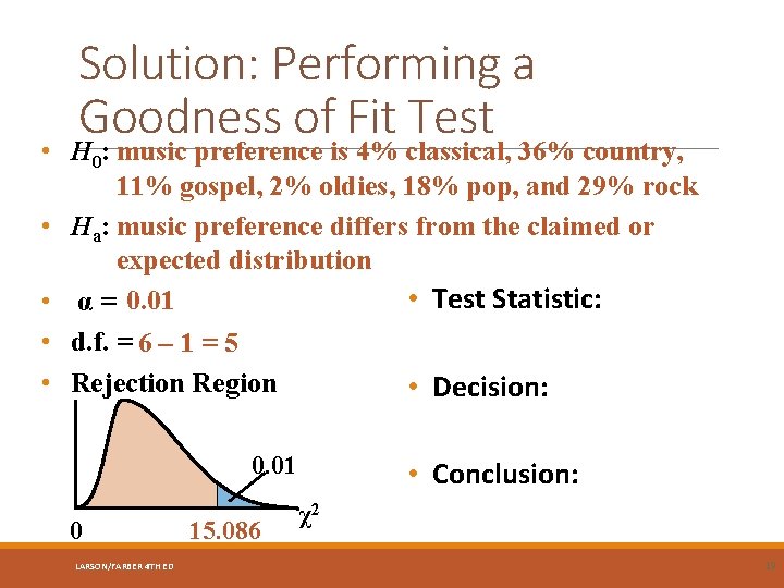
Solution: Performing a Goodness of Fit Test • H 0: music preference is 4% classical, 36% country, 11% gospel, 2% oldies, 18% pop, and 29% rock • Ha: music preference differs from the claimed or expected distribution • Test Statistic: • α = 0. 01 • d. f. = 6 – 1 = 5 • Rejection Region • Decision: 0. 01 0 LARSON/FARBER 4 TH ED 15. 086 • Conclusion: χ2 19

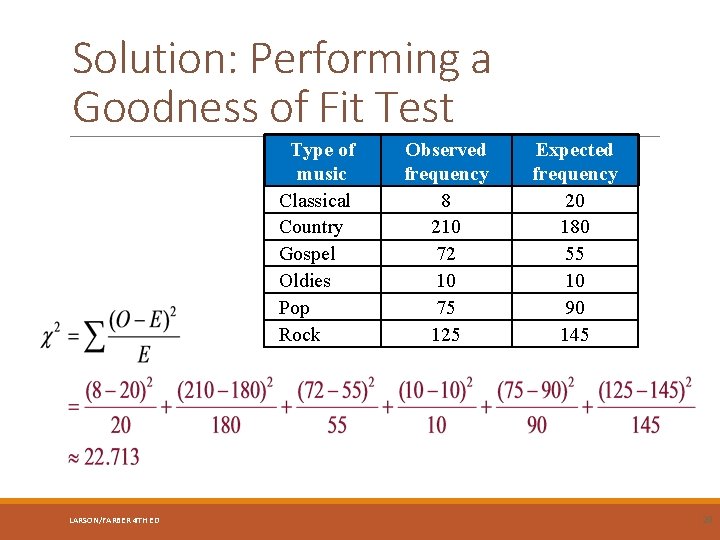
Solution: Performing a Goodness of Fit Test Type of music Classical Country Gospel Oldies Pop Rock LARSON/FARBER 4 TH ED Observed frequency 8 210 72 10 75 125 Expected frequency 20 180 55 10 90 145 20

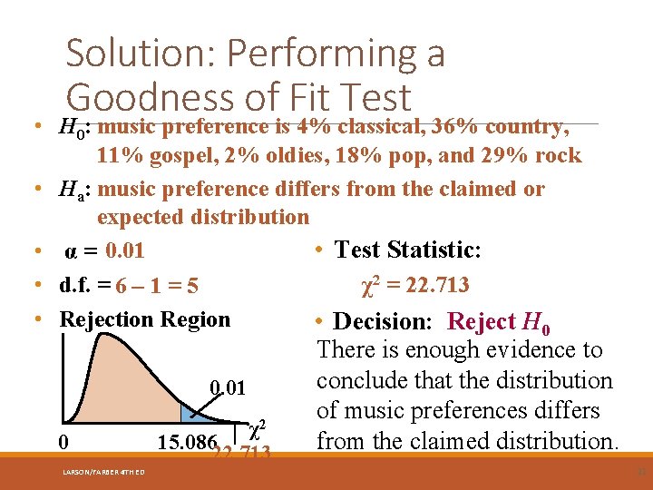
Solution: Performing a Goodness of Fit Test • H 0: music preference is 4% classical, 36% country, 11% gospel, 2% oldies, 18% pop, and 29% rock • Ha: music preference differs from the claimed or expected distribution • Test Statistic: • α = 0. 01 χ2 = 22. 713 • d. f. = 6 – 1 = 5 • Rejection Region • Decision: Reject H 0 0. 01 0 LARSON/FARBER 4 TH ED χ2 15. 086 22. 713 There is enough evidence to conclude that the distribution of music preferences differs from the claimed distribution. 21

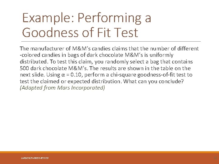
Example: Performing a Goodness of Fit Test The manufacturer of M&M’s candies claims that the number of different -colored candies in bags of dark chocolate M&M’s is uniformly distributed. To test this claim, you randomly select a bag that contains 500 dark chocolate M&M’s. The results are shown in the table on the next slide. Using α = 0. 10, perform a chi-square goodness-of-fit test to test the claimed or expected distribution. What can you conclude? (Adapted from Mars Incorporated) LARSON/FARBER 4 TH ED 22

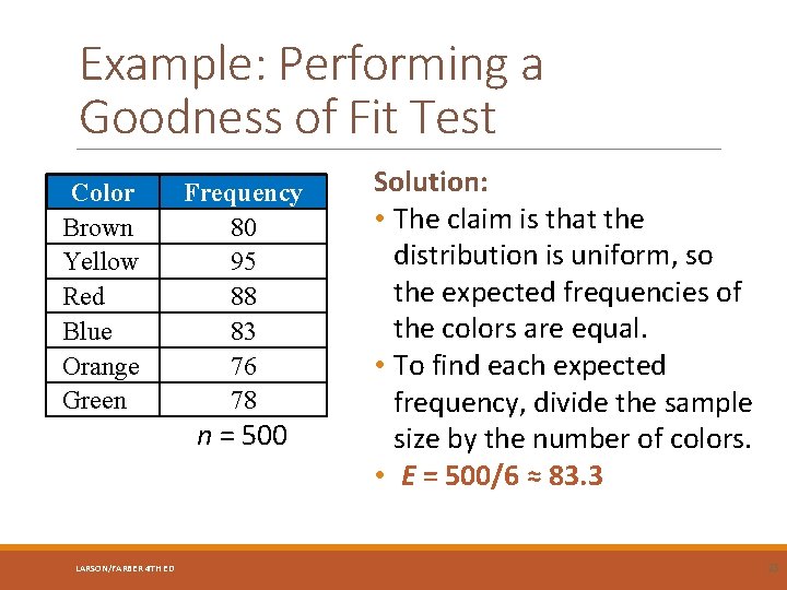
Example: Performing a Goodness of Fit Test Color Brown Yellow Red Blue Orange Green Frequency 80 95 88 83 76 78 n = 500 LARSON/FARBER 4 TH ED Solution: • The claim is that the distribution is uniform, so the expected frequencies of the colors are equal. • To find each expected frequency, divide the sample size by the number of colors. • E = 500/6 ≈ 83. 3 23

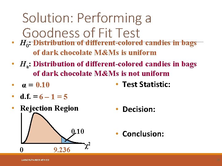
Solution: Performing a Goodness of Fit Test • H 0: Distribution of different-colored candies in bags of dark chocolate M&Ms is uniform • Ha: Distribution of different-colored candies in bags of dark chocolate M&Ms is not uniform • Test Statistic: • α = 0. 10 • d. f. = 6 – 1 = 5 • Rejection Region • Decision: 0. 10 0 LARSON/FARBER 4 TH ED 9. 236 • Conclusion: χ2 24

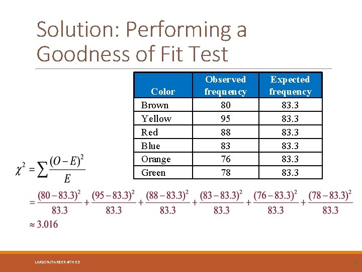
Solution: Performing a Goodness of Fit Test Color Brown Yellow Red Blue Orange Green LARSON/FARBER 4 TH ED Observed frequency 80 95 88 83 76 78 Expected frequency 83. 3 25

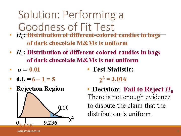
Solution: Performing a Goodness of Fit Test • H 0: Distribution of different-colored candies in bags of dark chocolate M&Ms is uniform • Ha: Distribution of different-colored candies in bags of dark chocolate M&Ms is not uniform • Test Statistic: • α = 0. 01 χ2 = 3. 016 • d. f. = 6 – 1 = 5 • Rejection Region • Decision: Fail to Reject H 0 0. 10 0 3. 016 LARSON/FARBER 4 TH ED 9. 236 χ2 There is not enough evidence to dispute the claim that the distribution is uniform. 26

Section 10. 1 Summary Used the chi-square distribution to test whether a frequency distribution fits a claimed distribution LARSON/FARBER 4 TH ED 27

Section 10. 2 INDEPENDENCE LARSON/FARBER 4 TH ED 28

Section 10. 2 Objectives Use a contingency table to find expected frequencies Use a chi-square distribution to test whether two variables are independent LARSON/FARBER 4 TH ED 29

Contingency Tables r c contingency table Shows the observed frequencies for two variables. The observed frequencies are arranged in r rows and c columns. The intersection of a row and a column is called a cell. LARSON/FARBER 4 TH ED 30

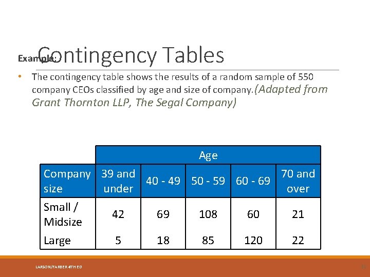
Contingency Tables Example: • The contingency table shows the results of a random sample of 550 company CEOs classified by age and size of company. (Adapted from Grant Thornton LLP, The Segal Company) Age Company 39 and 70 and 40 - 49 50 - 59 60 - 69 size under over Small / Midsize 42 69 108 60 21 Large 5 18 85 120 22 LARSON/FARBER 4 TH ED 31

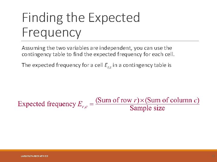
Finding the Expected Frequency Assuming the two variables are independent, you can use the contingency table to find the expected frequency for each cell. The expected frequency for a cell Er, c in a contingency table is LARSON/FARBER 4 TH ED 32

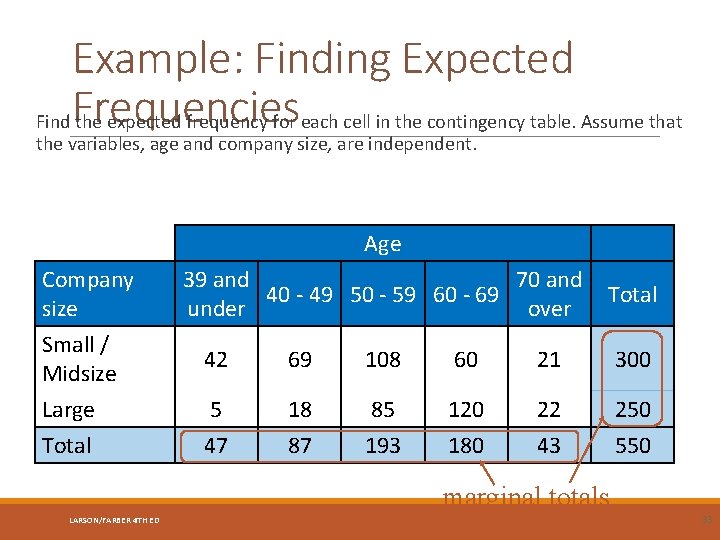
Example: Finding Expected Find Frequencies the expected frequency for each cell in the contingency table. Assume that the variables, age and company size, are independent. Age Company size 39 and 70 and 40 - 49 50 - 59 60 - 69 under over Total Small / Midsize 42 69 108 60 21 300 Large 5 18 85 120 22 250 Total 47 87 193 180 43 550 marginal totals LARSON/FARBER 4 TH ED 33

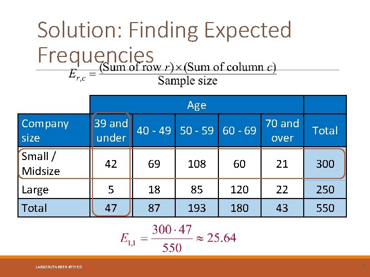
Solution: Finding Expected Frequencies Age Company size 39 and 70 and 40 - 49 50 - 59 60 - 69 under over Total Small / Midsize 42 69 108 60 21 300 Large 5 18 85 120 22 250 Total 47 87 193 180 43 550 LARSON/FARBER 4 TH ED 34

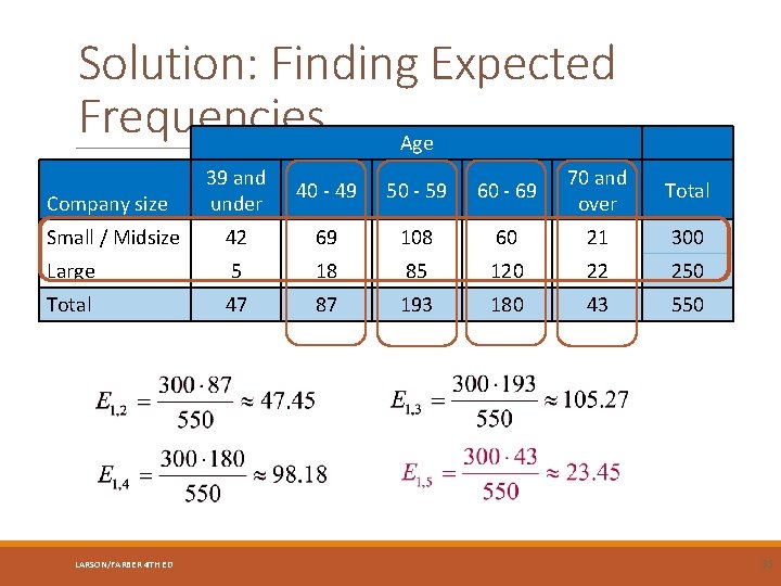
Solution: Finding Expected Frequencies Age Company size 39 and under 40 - 49 50 - 59 60 - 69 70 and over Total Small / Midsize 42 69 108 60 21 300 Large 5 18 85 120 22 250 Total 47 87 193 180 43 550 LARSON/FARBER 4 TH ED 35

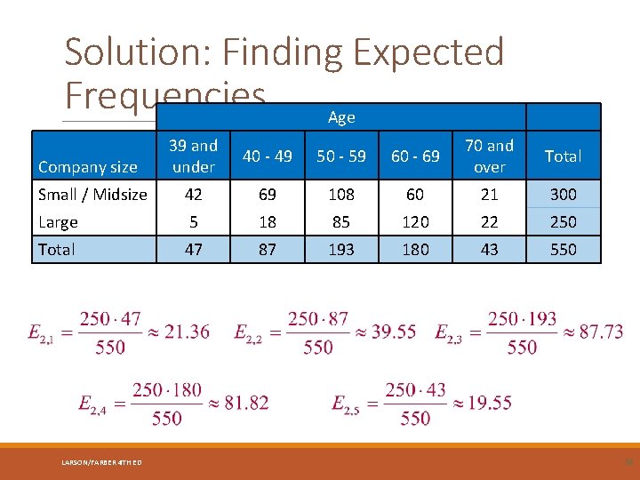
Solution: Finding Expected Frequencies Age Company size 39 and under 40 - 49 50 - 59 60 - 69 70 and over Total Small / Midsize 42 69 108 60 21 300 Large 5 18 85 120 22 250 Total 47 87 193 180 43 550 LARSON/FARBER 4 TH ED 36

Chi-Square Independence Test Chi-square independence test Used to test the independence of two variables. Can determine whether the occurrence of one variable affects the probability of the occurrence of the other variable. LARSON/FARBER 4 TH ED 37

Chi-Square Independence Test For the chi-square independence test to be used, the following must be true. 1. The observed frequencies must be obtained by using a random sample. 2. Each expected frequency must be greater than or equal to 5. LARSON/FARBER 4 TH ED 38

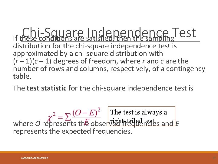
Chi-Square Independence Test If these conditions are satisfied, then the sampling distribution for the chi-square independence test is approximated by a chi-square distribution with (r – 1)(c – 1) degrees of freedom, where r and c are the number of rows and columns, respectively, of a contingency table. The test statistic for the chi-square independence test is The test is always a right-tailed test. and E where O represents the observed frequencies represents the expected frequencies. LARSON/FARBER 4 TH ED 39

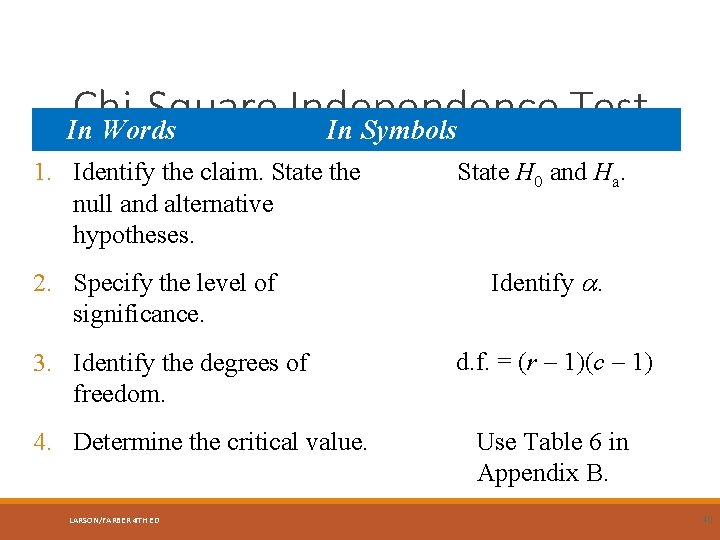
Chi-Square Independence Test In Words In Symbols 1. Identify the claim. State the null and alternative hypotheses. 2. Specify the level of significance. 3. Identify the degrees of freedom. 4. Determine the critical value. LARSON/FARBER 4 TH ED State H 0 and Ha. Identify . d. f. = (r – 1)(c – 1) Use Table 6 in Appendix B. 40

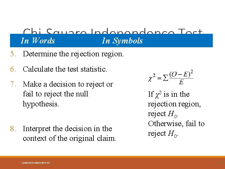
Chi-Square Independence Test In Words In Symbols 5. Determine the rejection region. 6. Calculate the test statistic. 7. Make a decision to reject or fail to reject the null hypothesis. 8. Interpret the decision in the context of the original claim. LARSON/FARBER 4 TH ED If χ2 is in the rejection region, reject H 0. Otherwise, fail to reject H 0. 41

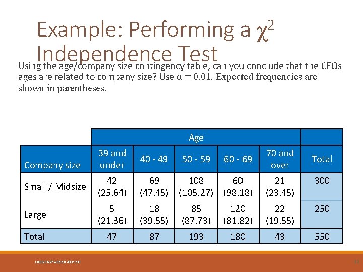
Example: Performing a Independence Test Using the age/company size contingency table, can you conclude that the CEOs 2 χ ages are related to company size? Use α = 0. 01. Expected frequencies are shown in parentheses. Age 39 and under 40 - 49 50 - 59 60 - 69 70 and over Small / Midsize 42 (25. 64) 69 (47. 45) 108 (105. 27) 60 (98. 18) 21 (23. 45) 300 Large 5 (21. 36) 18 (39. 55) 85 (87. 73) 120 (81. 82) 22 (19. 55) 250 Total 47 87 193 180 43 550 Company size LARSON/FARBER 4 TH ED Total 42

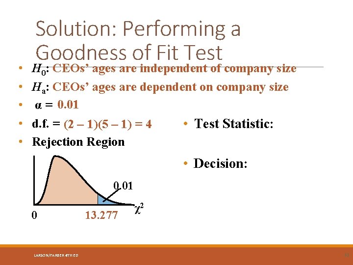
• • • Solution: Performing a Goodness of Fit Test H 0: CEOs’ ages are independent of company size Ha: CEOs’ ages are dependent on company size α = 0. 01 d. f. = (2 – 1)(5 – 1) = 4 • Test Statistic: Rejection Region • Decision: 0. 01 0 LARSON/FARBER 4 TH ED 13. 277 χ2 43

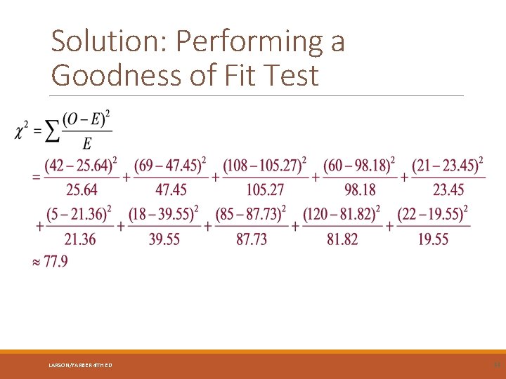
Solution: Performing a Goodness of Fit Test LARSON/FARBER 4 TH ED 44

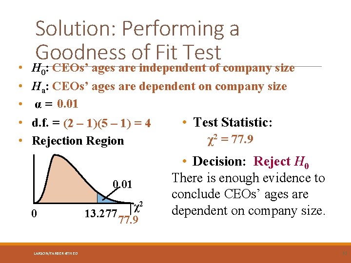
• • • Solution: Performing a Goodness of Fit Test H 0: CEOs’ ages are independent of company size Ha: CEOs’ ages are dependent on company size α = 0. 01 d. f. = (2 – 1)(5 – 1) = 4 • Test Statistic: χ2 = 77. 9 Rejection Region 0. 01 0 LARSON/FARBER 4 TH ED χ2 13. 277 77. 9 • Decision: Reject H 0 There is enough evidence to conclude CEOs’ ages are dependent on company size. 45

Section 10. 2 Summary Used a contingency table to find expected frequencies Used a chi-square distribution to test whether two variables are independent LARSON/FARBER 4 TH ED 46

Section 10. 3 COMPARING TWO VARIANCES LARSON/FARBER 4 TH ED 47

Section 10. 3 Objectives Interpret the F-distribution and use an F-table to find critical values Perform a two-sample F-test to compare two variances LARSON/FARBER 4 TH ED 48

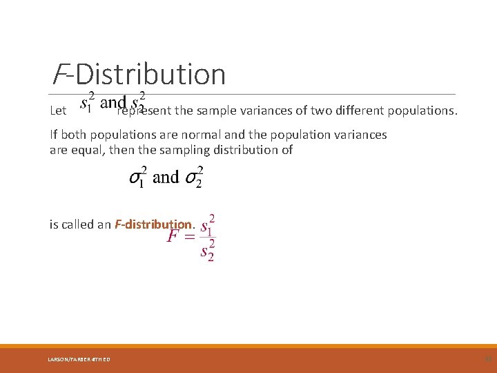
F-Distribution Let represent the sample variances of two different populations. If both populations are normal and the population variances are equal, then the sampling distribution of is called an F-distribution. LARSON/FARBER 4 TH ED 49

Properties of the FDistribution 1. The F-distribution is a family of curves each of which is determined by two types of degrees of freedom: ◦ ◦ The degrees of freedom corresponding to the variance in the numerator, denoted d. f. N The degrees of freedom corresponding to the variance in the denominator, denoted d. f. D 2. F-distributions are positively skewed. 3. The total area under each curve of an F-distribution is equal to 1. LARSON/FARBER 4 TH ED 50

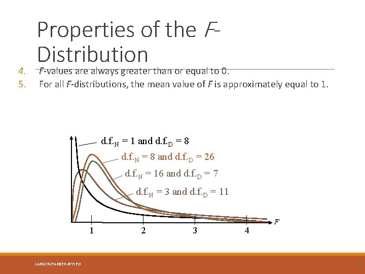
4. 5. Properties of the FDistribution F-values are always greater than or equal to 0. For all F-distributions, the mean value of F is approximately equal to 1. d. f. N = 1 and d. f. D = 8 d. f. N = 8 and d. f. D = 26 d. f. N = 16 and d. f. D = 7 d. f. N = 3 and d. f. D = 11 1 LARSON/FARBER 4 TH ED 2 3 4 F 51

Critical Values for the FDistribution 1. Specify the level of significance . 2. Determine the degrees of freedom for the numerator, d. f. N. 3. Determine the degrees of freedom for the denominator, d. f. D. 4. Use Table 7 in Appendix B to find the critical value. If the hypothesis test is a. one-tailed, use the F-table. b. two-tailed, use the ½ F-table. LARSON/FARBER 4 TH ED 52

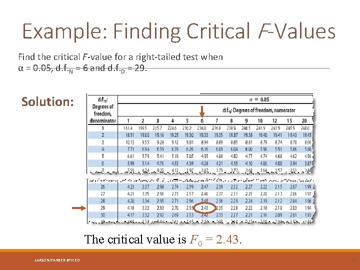
Example: Finding Critical F-Values Find the critical F-value for a right-tailed test when α = 0. 05, d. f. N = 6 and d. f. D = 29. Solution: The critical value is F 0 = 2. 43. LARSON/FARBER 4 TH ED 53

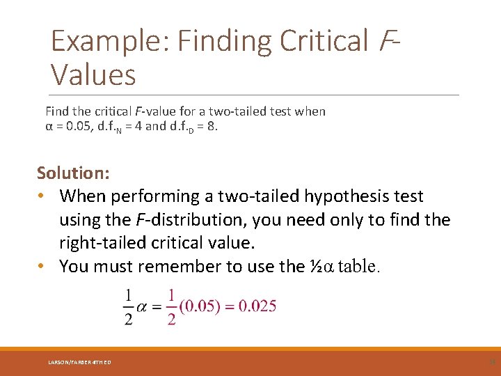
Example: Finding Critical FValues Find the critical F-value for a two-tailed test when α = 0. 05, d. f. N = 4 and d. f. D = 8. Solution: • When performing a two-tailed hypothesis test using the F-distribution, you need only to find the right-tailed critical value. • You must remember to use the ½α table. LARSON/FARBER 4 TH ED 54

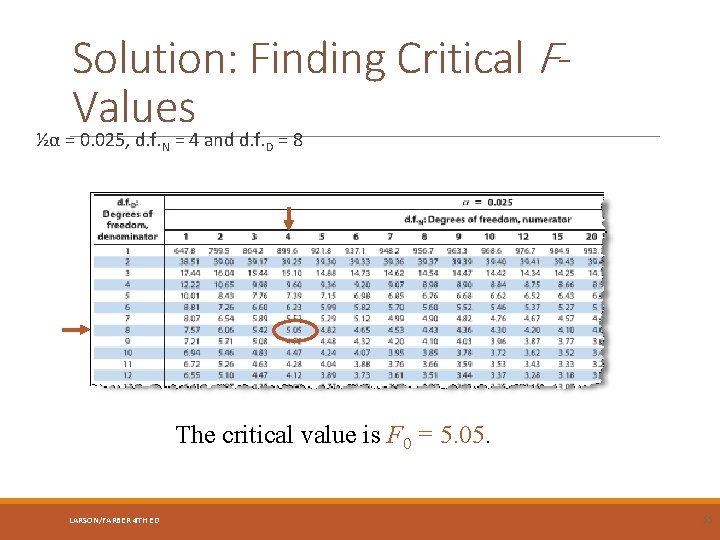
Solution: Finding Critical FValues ½α = 0. 025, d. f. N = 4 and d. f. D = 8 The critical value is F 0 = 5. 05. LARSON/FARBER 4 TH ED 55

Two-Sample F-Test for Variances To use the two-sample F-test for comparing two population variances, the following must be true. 1. The samples must be randomly selected. 2. The samples must be independent. 3. Each population must have a normal distribution. LARSON/FARBER 4 TH ED 56

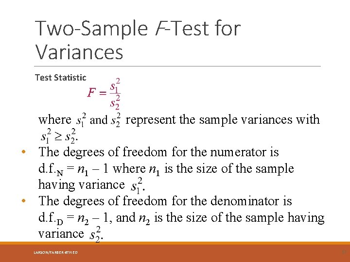
Two-Sample F-Test for Variances Test Statistic where represent the sample variances with • The degrees of freedom for the numerator is d. f. N = n 1 – 1 where n 1 is the size of the sample having variance • The degrees of freedom for the denominator is d. f. D = n 2 – 1, and n 2 is the size of the sample having variance LARSON/FARBER 4 TH ED 57

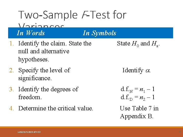
Two-Sample F-Test for Variances In Words In Symbols 1. Identify the claim. State the null and alternative hypotheses. State H 0 and Ha. 2. Specify the level of significance. Identify . 3. Identify the degrees of freedom. d. f. N = n 1 – 1 d. f. D = n 2 – 1 4. Determine the critical value. Use Table 7 in Appendix B. LARSON/FARBER 4 TH ED 58

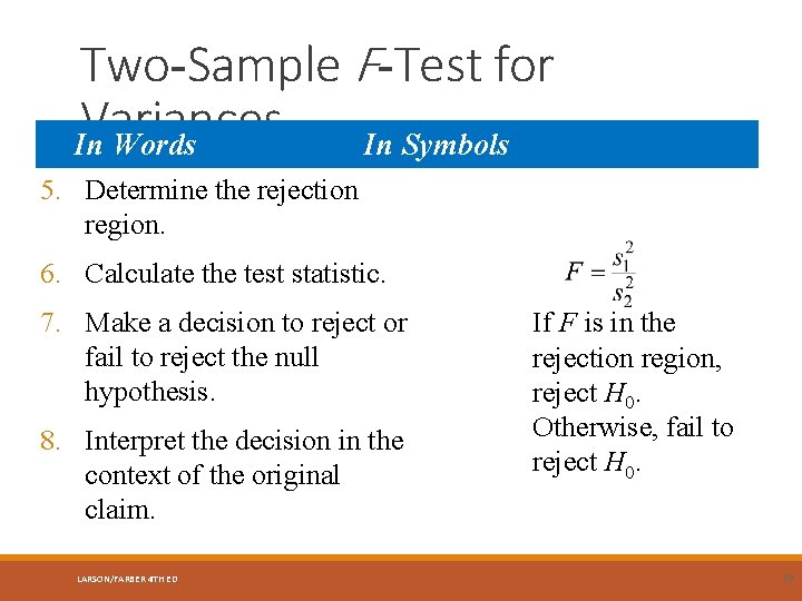
Two-Sample F-Test for Variances In Words In Symbols 5. Determine the rejection region. 6. Calculate the test statistic. 7. Make a decision to reject or fail to reject the null hypothesis. 8. Interpret the decision in the context of the original claim. LARSON/FARBER 4 TH ED If F is in the rejection region, reject H 0. Otherwise, fail to reject H 0. 59

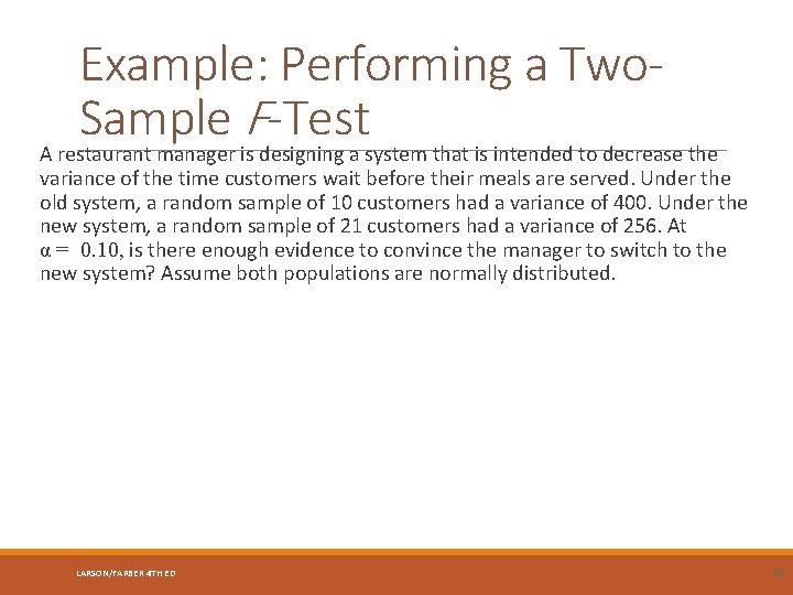
Example: Performing a Two. Sample F-Test A restaurant manager is designing a system that is intended to decrease the variance of the time customers wait before their meals are served. Under the old system, a random sample of 10 customers had a variance of 400. Under the new system, a random sample of 21 customers had a variance of 256. At α = 0. 10, is there enough evidence to convince the manager to switch to the new system? Assume both populations are normally distributed. LARSON/FARBER 4 TH ED 60

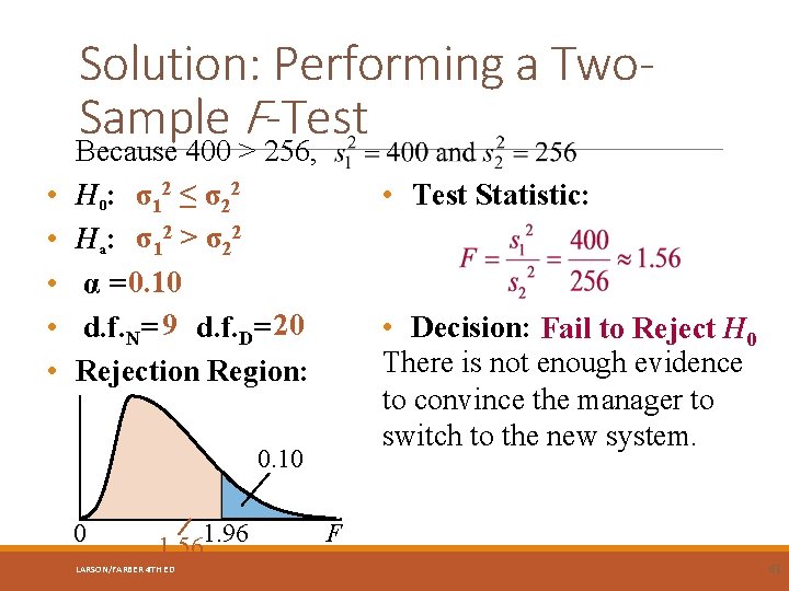
Solution: Performing a Two. Sample F-Test • • • Because 400 > 256, H 0: σ12 ≤ σ22 Ha: σ12 > σ22 α = 0. 10 d. f. N= 9 d. f. D= 20 Rejection Region: • Test Statistic: • Decision: Fail to Reject H 0 There is not enough evidence to convince the manager to switch to the new system. 0. 10 0 1. 561. 96 LARSON/FARBER 4 TH ED F 61

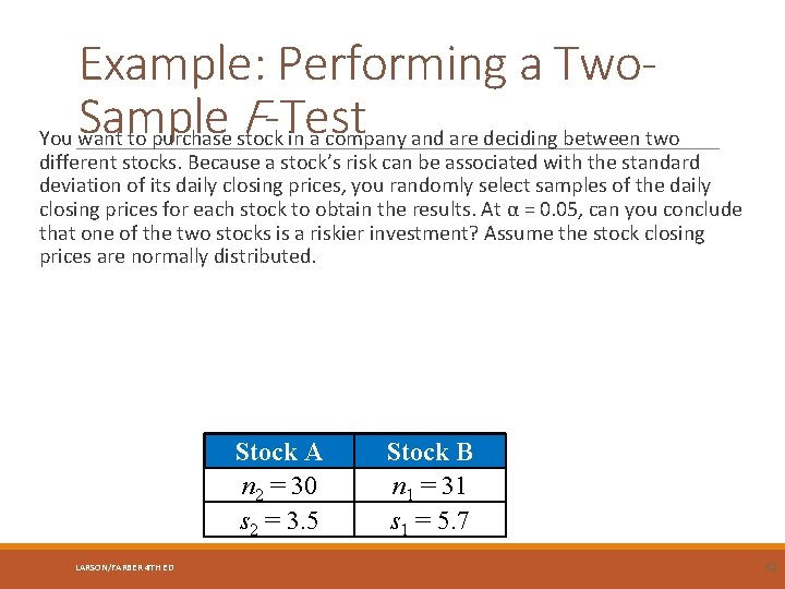
Example: Performing a Two. Sample F-Test You want to purchase stock in a company and are deciding between two different stocks. Because a stock’s risk can be associated with the standard deviation of its daily closing prices, you randomly select samples of the daily closing prices for each stock to obtain the results. At α = 0. 05, can you conclude that one of the two stocks is a riskier investment? Assume the stock closing prices are normally distributed. Stock A n 2 = 30 s 2 = 3. 5 LARSON/FARBER 4 TH ED Stock B n 1 = 31 s 1 = 5. 7 62

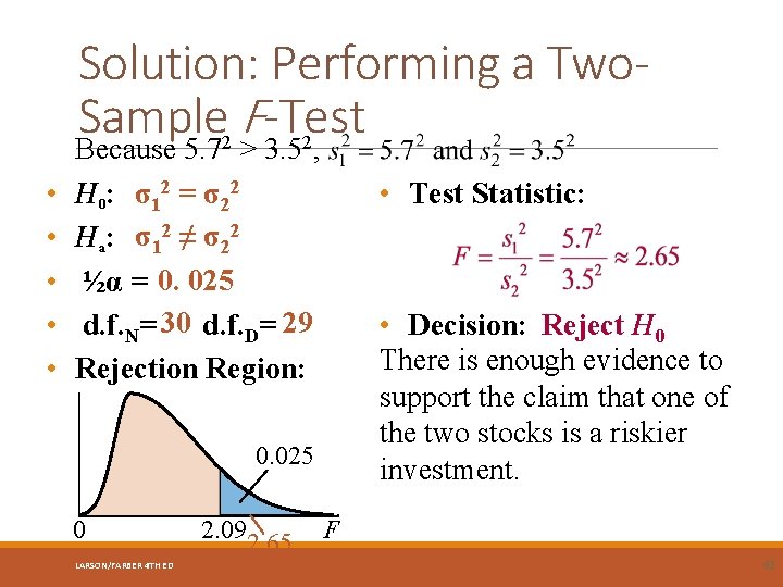
Solution: Performing a Two. Sample F -Test Because 5. 7 > 3. 5 , 2 • • • 2 • Test Statistic: H 0: σ12 = σ22 Ha: σ12 ≠ σ22 ½α = 0. 025 d. f. N= 30 d. f. D= 29 Rejection Region: • Decision: Reject H 0 There is enough evidence to support the claim that one of the two stocks is a riskier investment. 0. 025 0 LARSON/FARBER 4 TH ED 2. 092. 65 F 63

Section 10. 3 Summary Interpreted the F-distribution and used an F-table to find critical values Performed a two-sample F-test to compare two variances LARSON/FARBER 4 TH ED 64

Section 10. 4 ANALYSIS OF VARIANCE LARSON/FARBER 4 TH ED 65

Section 10. 4 Objectives Use one-way analysis of variance to test claims involving three or more means Introduce two-way analysis of variance LARSON/FARBER 4 TH ED 66

One-Way ANOVA One-way analysis of variance A hypothesis-testing technique that is used to compare means from three or more populations. Analysis of variance is usually abbreviated ANOVA. Hypotheses: ◦ H 0: μ 1 = μ 2 = μ 3 =…= μk (all population means are equal) ◦ Ha: At least one of the means is different from the others. LARSON/FARBER 4 TH ED 67

One-Way ANOVA In a one-way ANOVA test, the following must be true. 1. Each sample must be randomly selected from a normal, or approximately normal, population. 2. The samples must be independent of each other. 3. Each population must have the same variance. LARSON/FARBER 4 TH ED 68

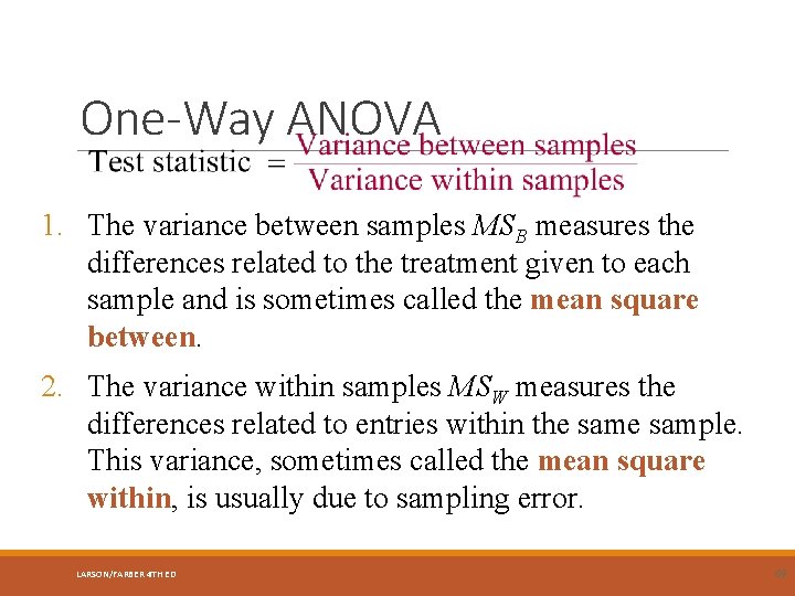
One-Way ANOVA 1. The variance between samples MSB measures the differences related to the treatment given to each sample and is sometimes called the mean square between. 2. The variance within samples MSW measures the differences related to entries within the sample. This variance, sometimes called the mean square within, is usually due to sampling error. LARSON/FARBER 4 TH ED 69

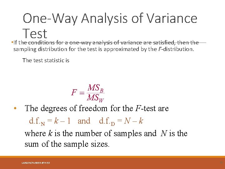
One-Way Analysis of Variance Test • If the conditions for a one-way analysis of variance are satisfied, then the sampling distribution for the test is approximated by the F-distribution. The test statistic is • The degrees of freedom for the F-test are d. f. N = k – 1 and d. f. D = N – k where k is the number of samples and N is the sum of the sample sizes. LARSON/FARBER 4 TH ED 70

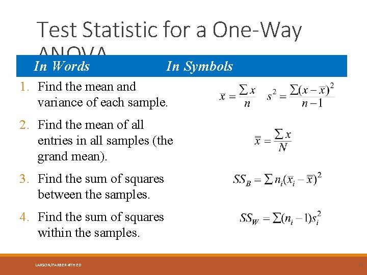
Test Statistic for a One-Way ANOVA In Words In Symbols 1. Find the mean and variance of each sample. 2. Find the mean of all entries in all samples (the grand mean). 3. Find the sum of squares between the samples. 4. Find the sum of squares within the samples. LARSON/FARBER 4 TH ED 71

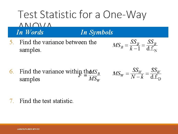
Test Statistic for a One-Way ANOVA In Words In Symbols 5. Find the variance between the samples. 6. Find the variance within the samples 7. Find the test statistic. LARSON/FARBER 4 TH ED 72

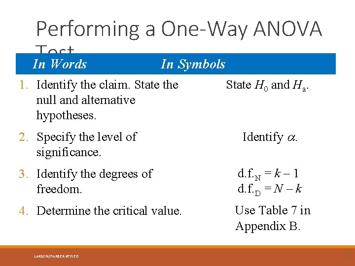
Performing a One-Way ANOVA Test In Words In Symbols 1. Identify the claim. State the null and alternative hypotheses. 2. Specify the level of significance. State H 0 and Ha. Identify . 3. Identify the degrees of freedom. d. f. N = k – 1 d. f. D = N – k 4. Determine the critical value. Use Table 7 in Appendix B. LARSON/FARBER 4 TH ED 73

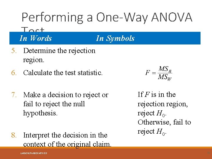
Performing a One-Way ANOVA Test In Words In Symbols 5. Determine the rejection region. 6. Calculate the test statistic. 7. Make a decision to reject or fail to reject the null hypothesis. 8. Interpret the decision in the context of the original claim. LARSON/FARBER 4 TH ED If F is in the rejection region, reject H 0. Otherwise, fail to reject H 0. 74

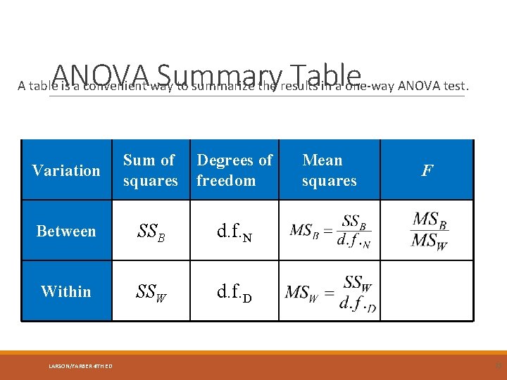
ANOVA Summary Table A table is a convenient way to summarize the results in a one-way ANOVA test. Variation Sum of squares Degrees of freedom Between SSB d. f. N Within SSW d. f. D LARSON/FARBER 4 TH ED Mean squares F 75

Example: Performing a One. Way ANOVA A medical researcher wants to determine whethere is a difference in the mean length of time it takes three types of pain relievers to provide relief from headache pain. Several headache sufferers are randomly selected and given one of the three medications. Each headache sufferer records the time (in minutes) it takes the medication to begin working. The results are shown on the next slide. At α = 0. 01, can you conclude that the mean times are different? Assume that each population of relief times is normally distributed and that the population variances are equal. LARSON/FARBER 4 TH ED 76

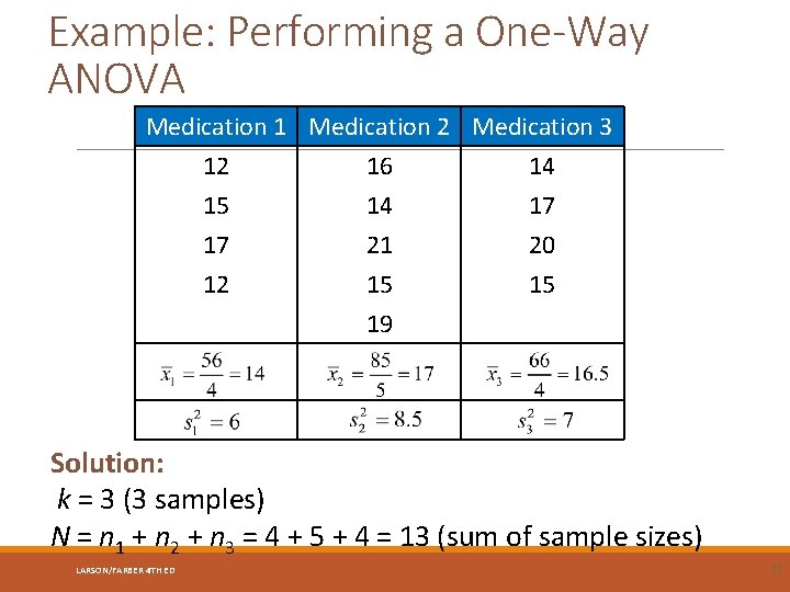
Example: Performing a One-Way ANOVA Medication 1 Medication 2 Medication 3 12 16 14 15 14 17 17 21 20 12 15 15 19 Solution: k = 3 (3 samples) N = n 1 + n 2 + n 3 = 4 + 5 + 4 = 13 (sum of sample sizes) LARSON/FARBER 4 TH ED 77

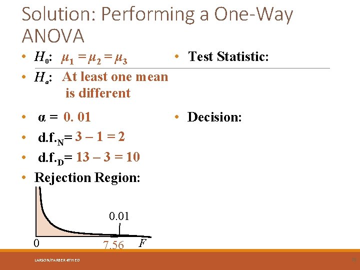
Solution: Performing a One-Way ANOVA • H 0 : μ 1 = μ 2 = μ 3 • Test Statistic: • Ha: At least one mean is different • • α = 0. 01 d. f. N= 3 – 1 = 2 d. f. D= 13 – 3 = 10 Rejection Region: • Decision: 0. 01 0 LARSON/FARBER 4 TH ED 7. 56 F 78

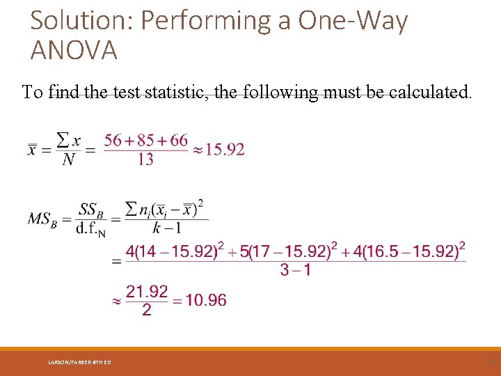
Solution: Performing a One-Way ANOVA To find the test statistic, the following must be calculated. LARSON/FARBER 4 TH ED 79

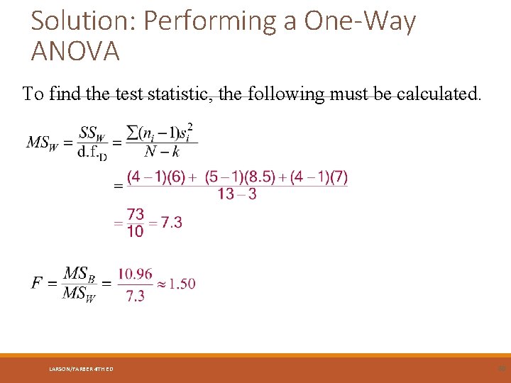
Solution: Performing a One-Way ANOVA To find the test statistic, the following must be calculated. LARSON/FARBER 4 TH ED 80

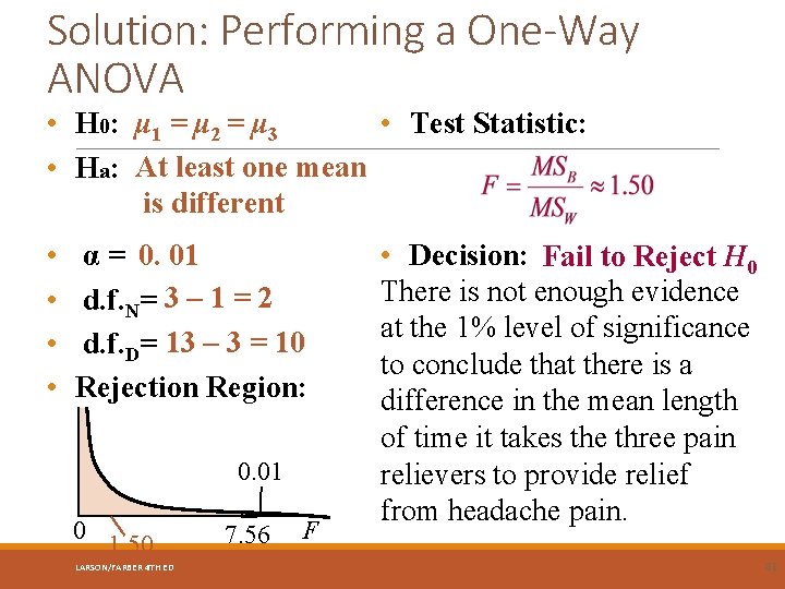
Solution: Performing a One-Way ANOVA • H 0: μ 1 = μ 2 = μ 3 • Test Statistic: • Ha: At least one mean is different • • α = 0. 01 d. f. N= 3 – 1 = 2 d. f. D= 13 – 3 = 10 Rejection Region: 0. 01 0 1. 50 LARSON/FARBER 4 TH ED 7. 56 F • Decision: Fail to Reject H 0 There is not enough evidence at the 1% level of significance to conclude that there is a difference in the mean length of time it takes the three pain relievers to provide relief from headache pain. 81

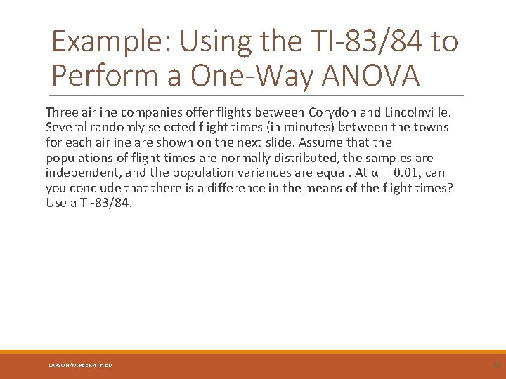
Example: Using the TI-83/84 to Perform a One-Way ANOVA Three airline companies offer flights between Corydon and Lincolnville. Several randomly selected flight times (in minutes) between the towns for each airline are shown on the next slide. Assume that the populations of flight times are normally distributed, the samples are independent, and the population variances are equal. At α = 0. 01, can you conclude that there is a difference in the means of the flight times? Use a TI-83/84. LARSON/FARBER 4 TH ED 82

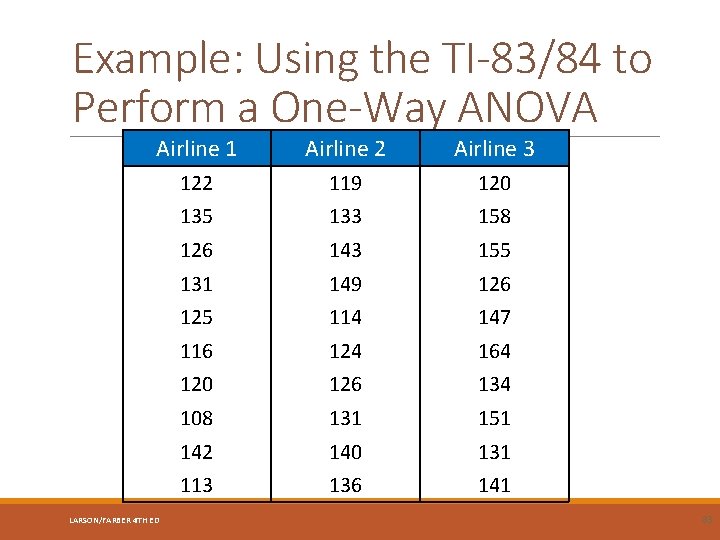
Example: Using the TI-83/84 to Perform a One-Way ANOVA Airline 1 Airline 2 Airline 3 122 119 120 135 133 158 126 143 155 131 149 126 125 114 147 116 124 164 120 126 134 108 131 151 142 140 131 113 136 141 LARSON/FARBER 4 TH ED 83

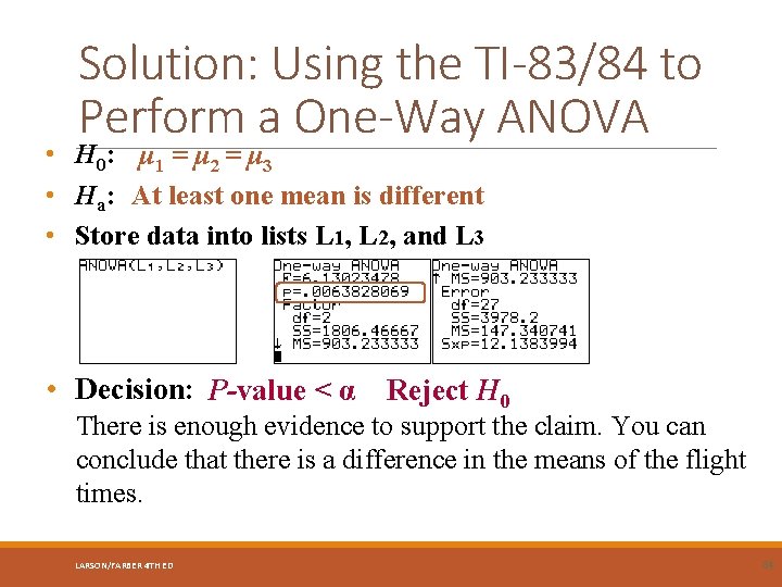
Solution: Using the TI-83/84 to Perform a One-Way ANOVA • H 0: μ 1 = μ 2 = μ 3 • Ha: At least one mean is different • Store data into lists L 1, L 2, and L 3 • Decision: P-value < α Reject H 0 There is enough evidence to support the claim. You can conclude that there is a difference in the means of the flight times. LARSON/FARBER 4 TH ED 84

Two-Way ANOVA Two-way analysis of variance A hypothesis-testing technique that is used to test the effect of two independent variables, or factors, on one dependent variable. LARSON/FARBER 4 TH ED 85

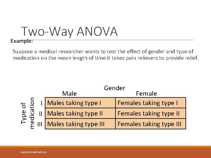
Two-Way ANOVA Example: Suppose a medical researcher wants to test the effect of gender and type of medication on the mean length of time it takes pain relievers to provide relief. Type of medication Gender Male I Males taking type I II Males taking type II III Males taking type III LARSON/FARBER 4 TH ED Females taking type III 86

Two-Way ANOVA Hypotheses Main effect The effect of one independent variable on the dependent variable. Interaction effect • The effect of both independent variables on the dependent variable. LARSON/FARBER 4 TH ED 87

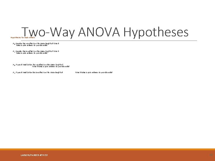
Two-Way ANOVA Hypotheses for main effects: H 0: Gender has no effect on the mean length of time it takes a pain reliever to provide relief. Ha: Gender has an effect on the mean length of time it takes a pain reliever to provide relief. H 0: Type of medication has no effect on the mean length of time it takes a pain reliever to provide relief. Ha: Type of medication has an effect on the mean length of LARSON/FARBER 4 TH ED time it takes a pain reliever to provide relief. 88

Two-Way ANOVA Hypotheses for interaction effects: H 0: There is no interaction effect between gender and type of medication on the mean length of time it takes a pain reliever to provide relief. Ha: There is an interaction effect between gender and type of medication on the mean length of time it takes a pain reliever to provide relief. LARSON/FARBER 4 TH ED 89

Two-Way ANOVA A two-way ANOVA test calculates an F-test statistic for each hypothesis. It is possible to reject none, two, or all of the null hypotheses. Can use a technology tool such as MINITAB to perform a twoway ANOVA test. LARSON/FARBER 4 TH ED 90

Section 10. 4 Summary Used one-way analysis of variance to test claims involving three or more means Introduced two-way analysis of variance LARSON/FARBER 4 TH ED 91