Chapter 10 Analysis of Variance Chapter 10 Chapter

Chapter 10 Analysis of Variance

Chapter 10 - Chapter Outcomes After studying the material in this chapter, you should be able to: • Recognize the applications that call for the use of analysis of variance. • Understand the logic of analysis of variance. • Be aware of several different analysis of variance designs and understand when to use each one. • Perform a single factor hypothesis test using analysis of variance manually and with the aid of Excel or Minitab software.

Chapter 10 - Chapter Outcomes (continued) After studying the material in this chapter, you should be able to: • Conduct and interpret post-analysis of variance pairwise comparisons procedures. • Recognize when randomized block analysis of variance is useful and be able to perform the randomized block analysis. • Perform two factor analysis of variance tests with replications using Excel or Minitab and interpret the output.

One-Way Analysis of Variance One-way analysis of variance is a design in which independent samples are obtained from k levels of a single factor for the purpose of testing whether the k levels have equal means.

One-Way Analysis of Variance A factor refers to a quantity under examination in an experiment as a possible cause of variation in the response variable.

One-Way Analysis of Variance Levels refer to the categories, measurements, or strata of a factor of interest in the current experiment.

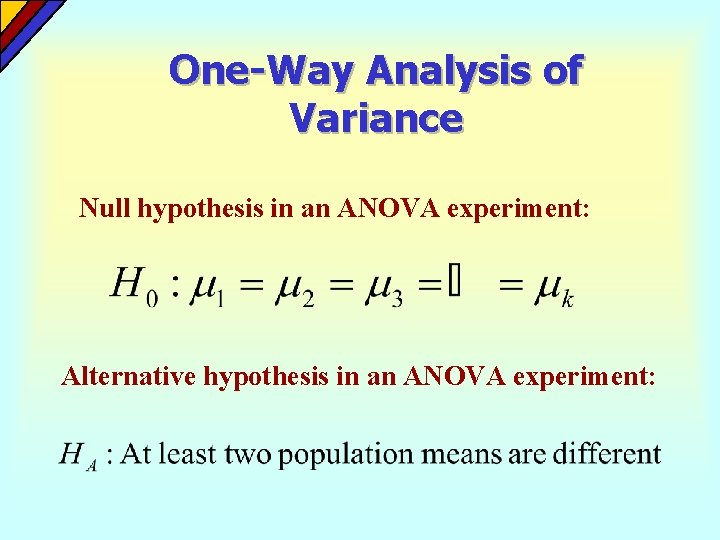
One-Way Analysis of Variance Null hypothesis in an ANOVA experiment: Alternative hypothesis in an ANOVA experiment:

One-Way Analysis of Variance COMPLETELY RANDOMIZED DESIGN An experiment is completely randomized if it consists of the independent random selection of observations representing each level of one factor.

One-Way Analysis of Variance BALANCED DESIGN An experiment is said to have a balanced design if the factor levels have equal sample sizes.

One-Way Analysis of Variance The ANOVA test is based on three assumptions: • All populations are normally distributed. • The population variances are equal. • The observations are independent, meaning that any one individual value is not dependent on the value of any other observation.

One-Way Analysis of Variance Total Variation The total variation in the data refers to the aggregate dispersion of the individual data values across the various factor levels.

One-Way Analysis of Variance Within-Sample Variation The dispersion that exists among the data values within a particular factor level is called the within-sample variation

One-Way Analysis of Variance Between-Sample Variation The dispersion among the factor sample means is called the between-sample variation

One-Way Analysis of Variance PARTITIONED SUM OF SQUARES where: TSS = Total Sum of Squares SSB = Sum of Squares Between SSW = Sum of Squares Within

One-Way Analysis of Variance Null hypothesis in an ANOVA experiment: Alternative hypothesis in an ANOVA experiment:

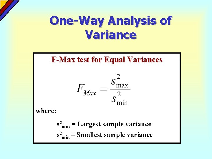
One-Way Analysis of Variance F-Max test for Equal Variances where: s 2 max = Largest sample variance s 2 min = Smallest sample variance

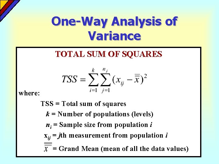
One-Way Analysis of Variance TOTAL SUM OF SQUARES where: TSS = Total sum of squares k = Number of populations (levels) ni = Sample size from population i xij = jth measurement from population i = Grand Mean (mean of all the data values)

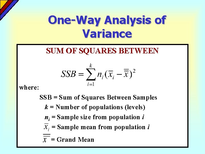
One-Way Analysis of Variance SUM OF SQUARES BETWEEN where: SSB = Sum of Squares Between Samples k = Number of populations (levels) ni = Sample size from population i = Sample mean from population i = Grand Mean

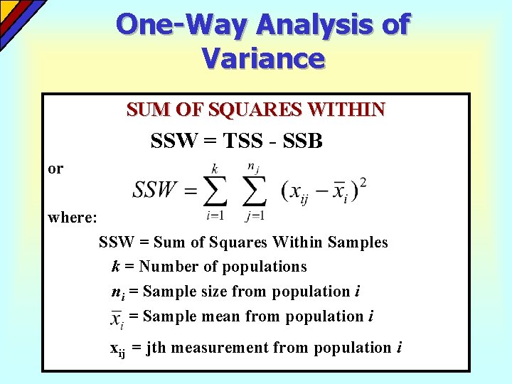
One-Way Analysis of Variance SUM OF SQUARES WITHIN SSW = TSS - SSB or where: SSW = Sum of Squares Within Samples k = Number of populations ni = Sample size from population i = Sample mean from population i xij = jth measurement from population i

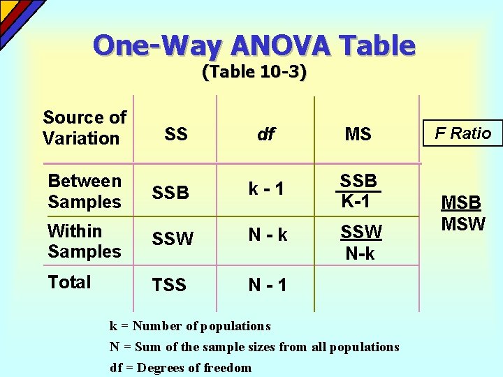
One-Way ANOVA Table (Table 10 -3) Source of Variation SS df MS SSB K-1 SSW N-k Between Samples SSB k-1 Within Samples SSW N-k Total TSS N-1 k = Number of populations N = Sum of the sample sizes from all populations df = Degrees of freedom F Ratio MSB MSW

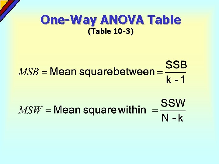
One-Way ANOVA Table (Table 10 -3)

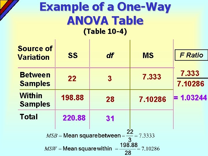
Example of a One-Way ANOVA Table (Table 10 -4) Source of Variation SS F Ratio df MS 7. 333 7. 10286 = 1. 03244 Between Samples 22 3 7. 333 Within Samples 198. 88 28 7. 10286 Total 220. 88 31

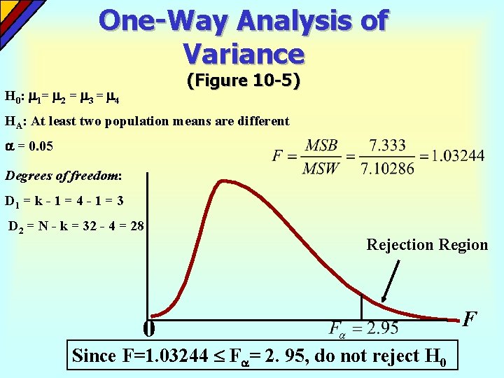
One-Way Analysis of Variance (Figure 10 -5) H 0 : 1 = 2 = 3 = 4 HA: At least two population means are different = 0. 05 Degrees of freedom: D 1 = k - 1 = 4 - 1 = 3 D 2 = N - k = 32 - 4 = 28 0 Rejection Region Since F=1. 03244 F = 2. 95, do not reject H 0 F

The Tukey-Kramer Procedure The Tukey-Kramer procedure is a method for testing which populations have different means, after the one-way ANOVA null hypothesis has been rejected.

The Tukey-Kramer Procedure and One-Way ANOVA The experiment-wide error rate is the proportion of experiments in which at least one of the set of confidence intervals constructed does not contain the true value of the population parameter being estimated.

The Tukey-Kramer Procedure and One-Way ANOVA TUKEY-KRAMER CRITICAL RANGE where: q = Value from standardized range table with k and N - k degrees of freedom for the desired level of . MSW = Mean Square Within ni and nj = Sample sizes from populations (levels) i and j, respectively.

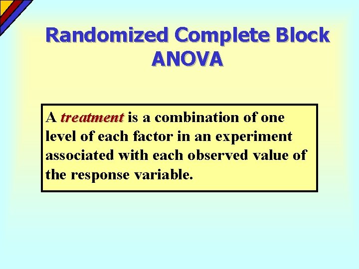
Randomized Complete Block ANOVA A treatment is a combination of one level of each factor in an experiment associated with each observed value of the response variable.

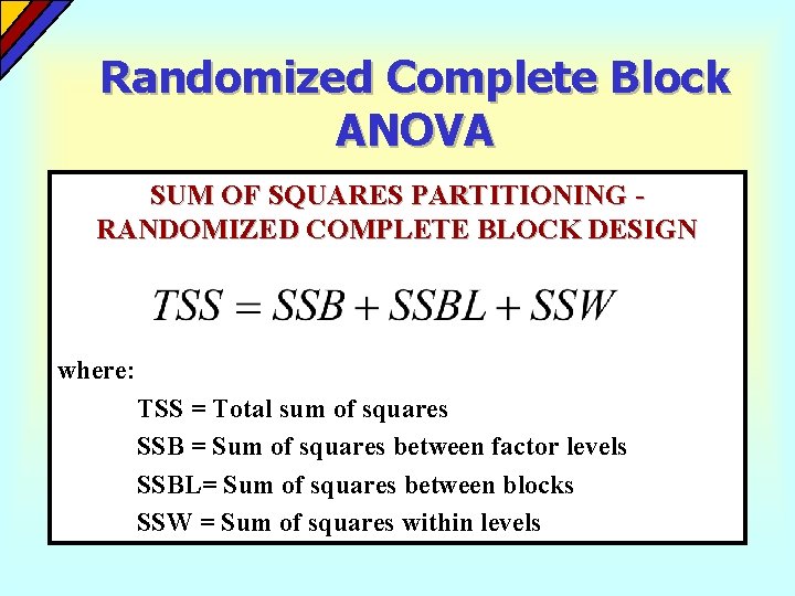
Randomized Complete Block ANOVA SUM OF SQUARES PARTITIONING RANDOMIZED COMPLETE BLOCK DESIGN where: TSS = Total sum of squares SSB = Sum of squares between factor levels SSBL= Sum of squares between blocks SSW = Sum of squares within levels

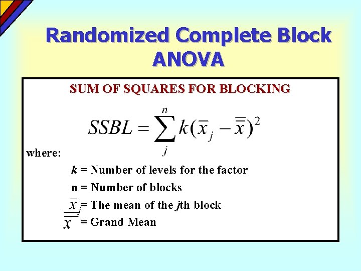
Randomized Complete Block ANOVA SUM OF SQUARES FOR BLOCKING where: k = Number of levels for the factor n = Number of blocks = The mean of the jth block = Grand Mean

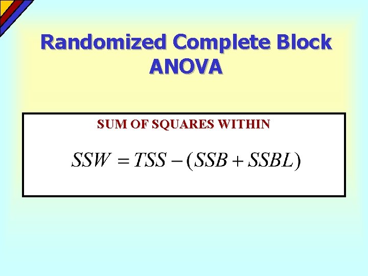
Randomized Complete Block ANOVA SUM OF SQUARES WITHIN

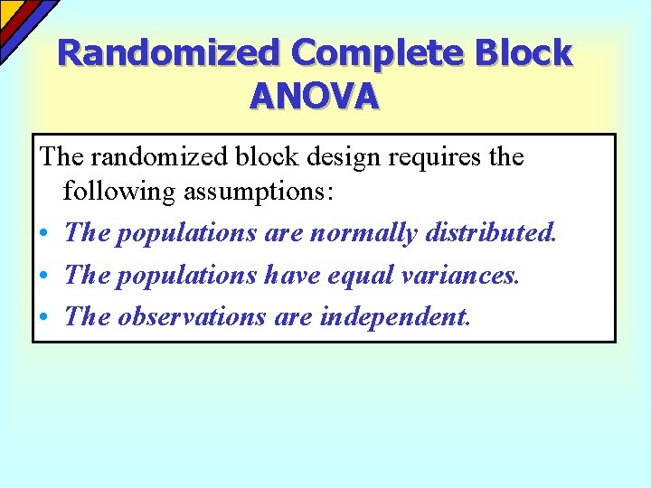
Randomized Complete Block ANOVA The randomized block design requires the following assumptions: • The populations are normally distributed. • The populations have equal variances. • The observations are independent.

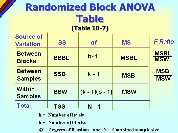
Randomized Block ANOVA Table (Table 10 -7) Source of Variation SS df Between Blocks SSBL b- 1 Between Samples SSB k-1 Within Samples SSW Total TSS (k - 1)(b - 1) MS F Ratio MSBL MSW MSB MSW N-1 k = Number of levels b = Number of blocks df = Degrees of freedom and N = Combined sample size

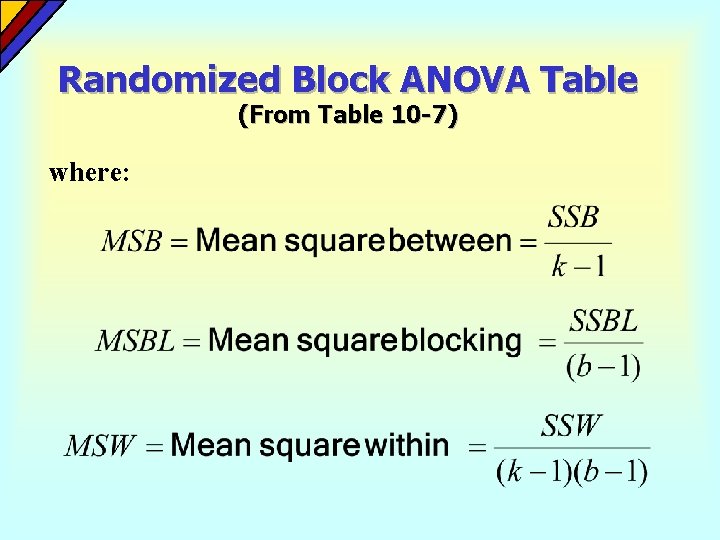
Randomized Block ANOVA Table (From Table 10 -7) where:

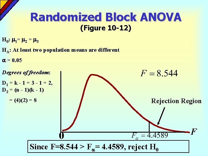
Randomized Block ANOVA (Figure 10 -12) H 0 : 1 = 2 = 3 HA: At least two population means are different = 0. 05 Degrees of freedom: D 1 = k - 1 = 3 - 1 = 2, D 2 = (n - 1)(k - 1) = (4)(2) = 8 Rejection Region 0 Since F=8. 544 > F = 4. 4589, reject H 0 F

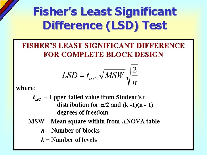
Fisher’s Least Significant Difference (LSD) Test FISHER’S LEAST SIGNIFICANT DIFFERENCE FOR COMPLETE BLOCK DESIGN where: t /2 = Upper-tailed value from Student’s tdistribution for /2 and (k -1)(n - 1) degrees of freedom MSW = Mean square within from ANOVA table n = Number of blocks k = Number of levels

Two-Factor Analysis of Variance Two-factor ANOVA is a technique used to analyze two factors in an analysis of variance framework.

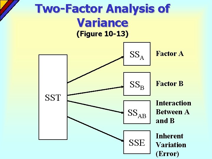
Two-Factor Analysis of Variance (Figure 10 -13) SSA Factor A SSB Factor B SST SSAB Interaction Between A and B SSE Inherent Variation (Error)

Two-Factor Analysis of Variance The necessary assumptions for the two factor ANOVA are: • The population values for each combination of pairwise factor levels are normally distributed. • The variances for each population are equal. • The samples are independent. • The observations are independent.

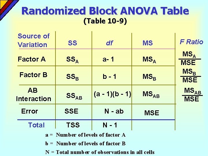
Randomized Block ANOVA Table (Table 10 -9) Source of Variation SS df MS Factor A SSA a- 1 MSA Factor B SSB b-1 MSB AB Interaction Error Total (a - 1)(b - 1) MSAB SSE N - ab MSE TSS N-1 SSAB a = Number of levels of factor A b = Number of levels of factor B N = Total number of observations in all cells F Ratio MSA MSE MSB MSE MSAB MSE

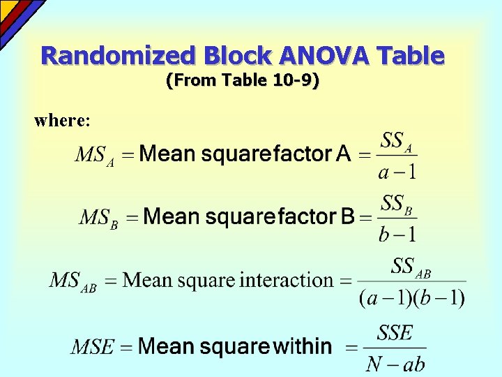
Randomized Block ANOVA Table (From Table 10 -9) where:

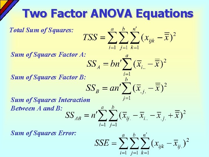
Two Factor ANOVA Equations Total Sum of Squares: Sum of Squares Factor A: Sum of Squares Factor B: Sum of Squares Interaction Between A and B: Sum of Squares Error:

Two Factor ANOVA Equations where: a = Number of levels of factor A b = Number of levels of factor B n’ = Number of replications in each cell

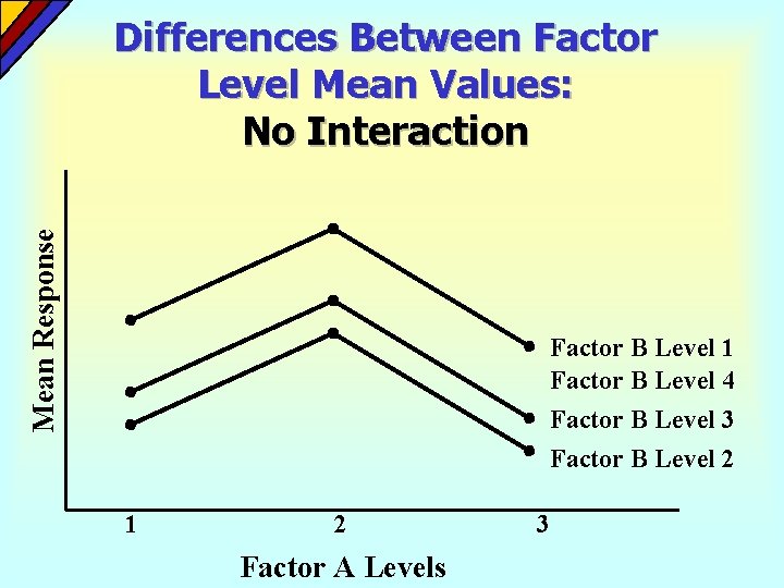
Mean Response Differences Between Factor Level Mean Values: No Interaction Factor B Level 1 Factor B Level 4 Factor B Level 3 Factor B Level 2 1 2 Factor A Levels 3

Mean Response Differences Between Factor Level Mean Values: Interaction Present Factor B Level 1 Factor B Level 2 Factor B Level 3 Factor B Level 4 1 2 Factor A Levels 3

A Caution About Interaction When conducting hypothesis tests for a two factor ANOVA: • Test for interaction. • If interaction is present conduct a one-way ANOVA to test the levels of one of the factors using only one level of the other factor. • If no interaction is found, test factor A and factor B.

Key Terms • Balanced Design • Between-Sample Variation • Completely Randomized Design • Experiment-Wide Error Rate • Factor • Levels • One-Way Analysis of Variance • Total Variation • Treatment • Within-Sample Variation