Chapter 10 11 Indexes v 10 Treestructured Indexes

Chapter 10, 11 Indexes v 10. Tree-structured Indexes § Intuition for tree indexes § ISAM: a static structure § B+ Trees • Operations • Search • Insert • Delete v 11. Hash-based Indexes § Static Hashing § Extendible Hashing • Directory • Insert • Delete § Linear Hashing • Special cases • When to split? • Key Compression • Bulk Loading • Order § Extendible vs. Linear Hashing • Updates may change rids 2/27/2021 PSU’s CS 587 1

Learning Objectives Describe the pros and cons of ISAM v Perform inserts and deletes on Btrees, extndible and linear hash indexes v For Btrees: Describe algorithms for bulk loading and key compression v Explain why hash indexes are rarely used v 2/27/2021 PSU’s CS 587 2

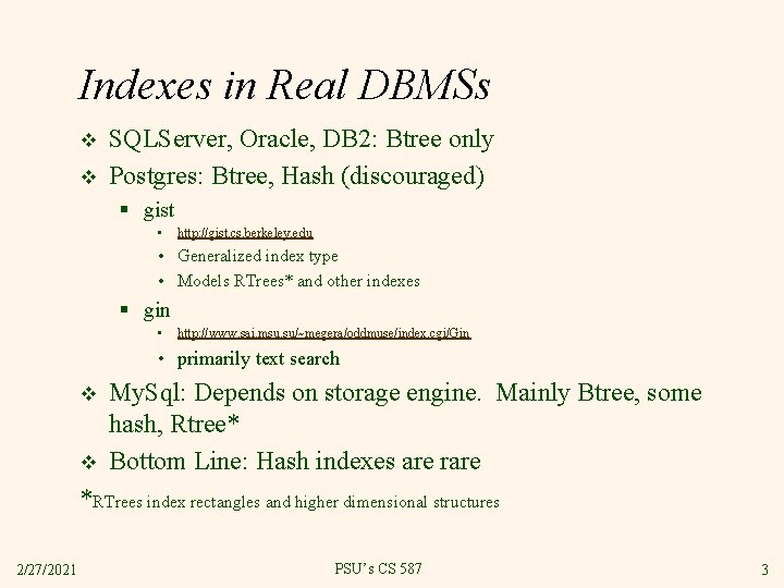
Indexes in Real DBMSs v v SQLServer, Oracle, DB 2: Btree only Postgres: Btree, Hash (discouraged) § gist • http: //gist. cs. berkeley. edu • Generalized index type • Models RTrees* and other indexes § gin • http: //www. sai. msu. su/~megera/oddmuse/index. cgi/Gin • primarily text search v v My. Sql: Depends on storage engine. Mainly Btree, some hash, Rtree* Bottom Line: Hash indexes are rare *RTrees index rectangles and higher dimensional structures 2/27/2021 PSU’s CS 587 3

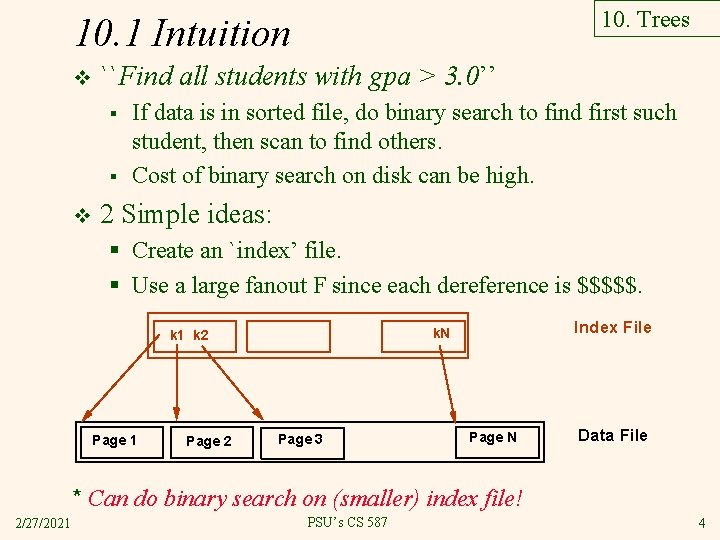
10. Trees 10. 1 Intuition v ``Find all students with gpa > 3. 0’’ § § v If data is in sorted file, do binary search to find first such student, then scan to find others. Cost of binary search on disk can be high. 2 Simple ideas: § Create an `index’ file. § Use a large fanout F since each dereference is $$$$$. Page 1 Page 2 Index File k. N k 1 k 2 Page 3 Page N Data File * Can do binary search on (smaller) index file! 2/27/2021 PSU’s CS 587 4

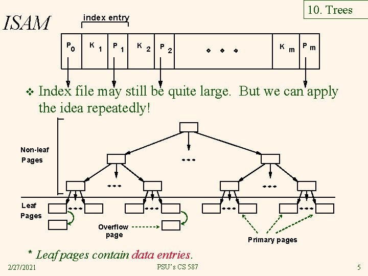
ISAM P 0 v 10. Trees index entry K 1 P 1 K 2 P 2 K m Pm Index file may still be quite large. But we can apply the idea repeatedly! Non-leaf Pages Leaf Pages Overflow page Primary pages * Leaf pages contain data entries. 2/27/2021 PSU’s CS 587 5

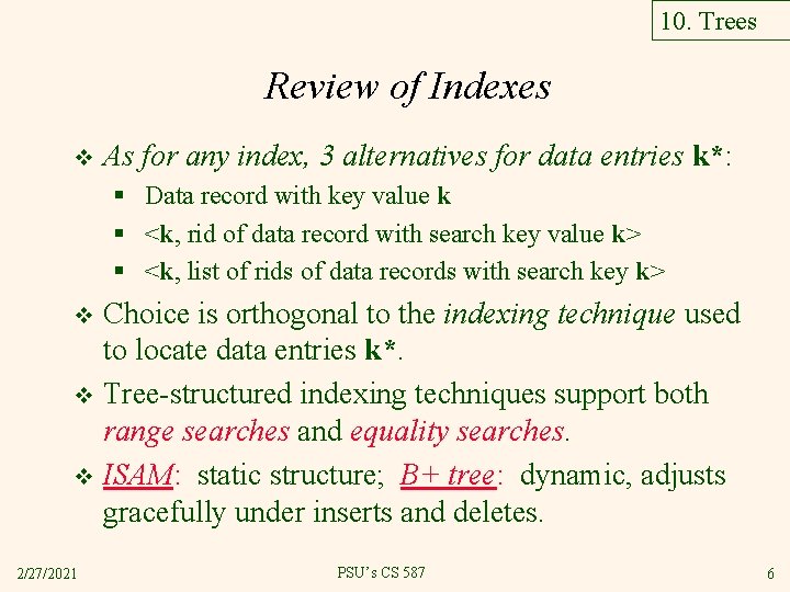
10. Trees Review of Indexes v As for any index, 3 alternatives for data entries k*: § Data record with key value k § <k, rid of data record with search key value k> § <k, list of rids of data records with search key k> Choice is orthogonal to the indexing technique used to locate data entries k*. v Tree-structured indexing techniques support both range searches and equality searches. v ISAM: static structure; B+ tree: dynamic, adjusts gracefully under inserts and deletes. v 2/27/2021 PSU’s CS 587 6

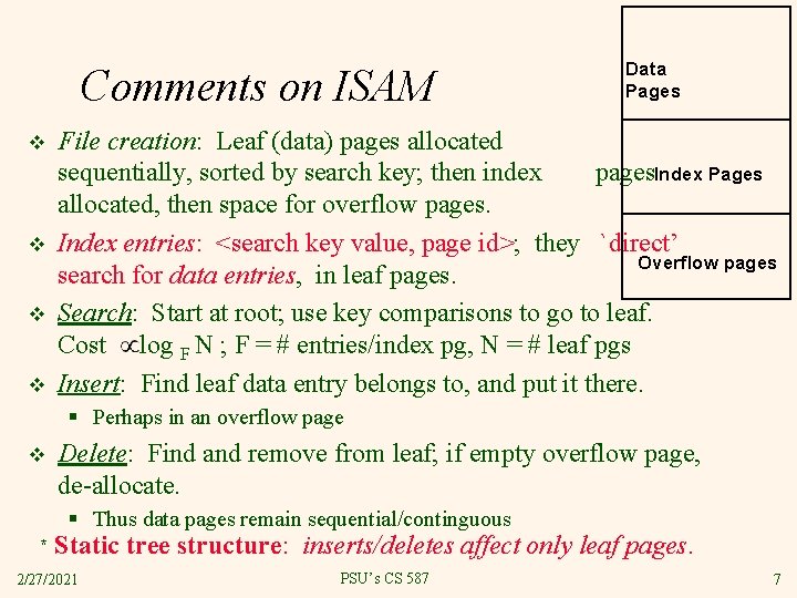
Comments on ISAM v v Data Pages File creation: Leaf (data) pages allocated sequentially, sorted by search key; then index pages. Index Pages allocated, then space for overflow pages. Index entries: <search key value, page id>; they `direct’ Overflow pages search for data entries, in leaf pages. Search: Start at root; use key comparisons to go to leaf. Cost log F N ; F = # entries/index pg, N = # leaf pgs Insert: Find leaf data entry belongs to, and put it there. § Perhaps in an overflow page v Delete: Find and remove from leaf; if empty overflow page, de-allocate. § Thus data pages remain sequential/continguous * Static tree structure: inserts/deletes affect only leaf pages. 2/27/2021 PSU’s CS 587 7

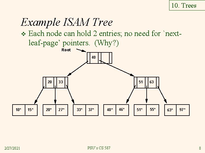
10. Trees Example ISAM Tree v Each node can hold 2 entries; no need for `nextleaf-page’ pointers. (Why? ) Root 40 10* 2/27/2021 15* 20 33 20* 27* 51 33* 37* 40* PSU’s CS 587 46* 51* 63 55* 63* 97* 8

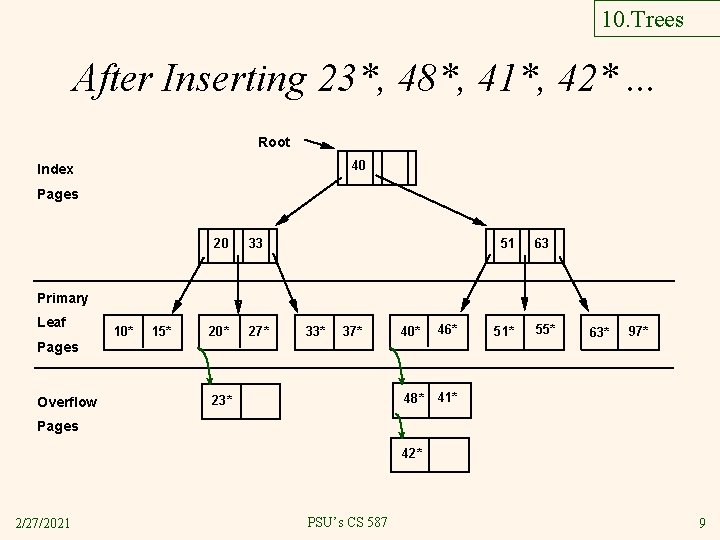
10. Trees After Inserting 23*, 48*, 41*, 42*. . . Root 40 Index Pages 20 33 20* 27* 51 63 Primary Leaf 10* 15* 33* 37* 40* 46* 48* 41* Pages Overflow 23* 51* 55* 63* 97* Pages 42* 2/27/2021 PSU’s CS 587 9

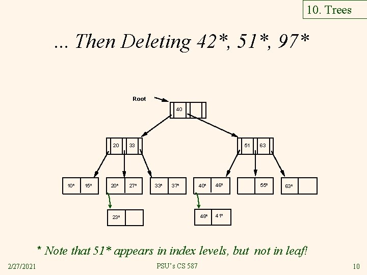
10. Trees . . . Then Deleting 42*, 51*, 97* Root 40 10* 15* 20 33 20* 27* 51 33* 37* 23* 40* 46* 48* 41* 63 55* 63* * Note that 51* appears in index levels, but not in leaf! 2/27/2021 PSU’s CS 587 10

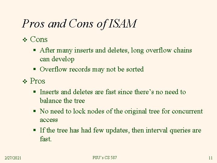
Pros and Cons of ISAM v Cons § After many inserts and deletes, long overflow chains can develop § Overflow records may not be sorted v Pros § Inserts and deletes are fast since there’s no need to balance the tree § No need to lock nodes of the original tree for concurrent access § If the tree has had few updates, then interval queries are fast. 2/27/2021 PSU’s CS 587 11

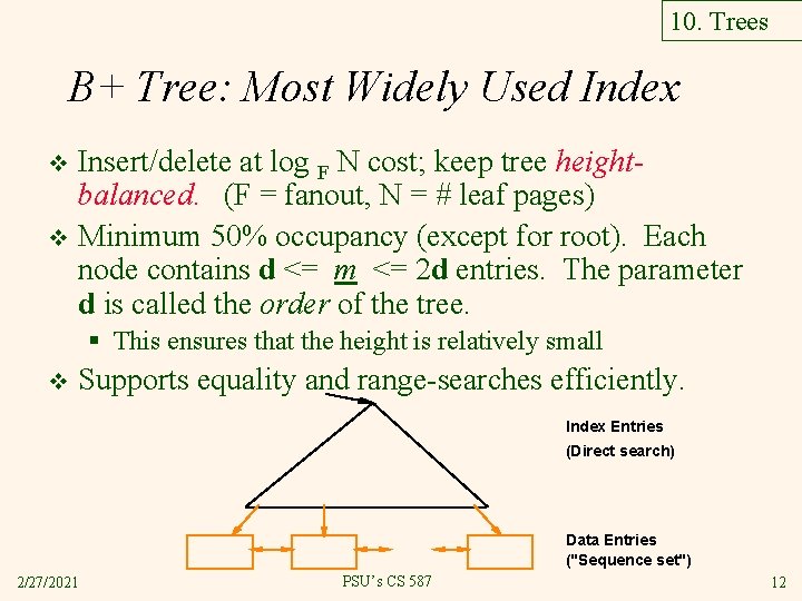
10. Trees B+ Tree: Most Widely Used Index Insert/delete at log F N cost; keep tree heightbalanced. (F = fanout, N = # leaf pages) v Minimum 50% occupancy (except for root). Each node contains d <= m <= 2 d entries. The parameter d is called the order of the tree. v § This ensures that the height is relatively small v Supports equality and range-searches efficiently. Index Entries (Direct search) Data Entries ("Sequence set") 2/27/2021 PSU’s CS 587 12

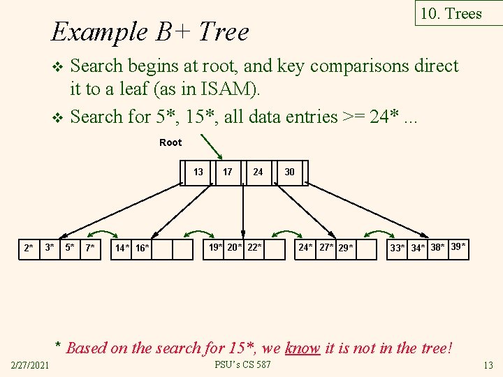
10. Trees Example B+ Tree Search begins at root, and key comparisons direct it to a leaf (as in ISAM). v Search for 5*, 15*, all data entries >= 24*. . . v Root 13 2* 3* 5* 7* 14* 16* 17 24 19* 20* 22* 30 24* 27* 29* 33* 34* 38* 39* * Based on the search for 15*, we know it is not in the tree! 2/27/2021 PSU’s CS 587 13

10. Trees Inserting a Data Entry into a B+ Tree Find correct leaf L. v Put data entry onto L. v § § If L has enough space, done! Else, must split L (into L and a new node L 2) • Redistribute entries evenly, copy up middle key. • Insert index entry pointing to L 2 into parent of L. v This can happen recursively § v Splits “grow” tree; root split increases height. § 2/27/2021 To split index node, redistribute entries evenly, but push up middle key. (Contrast with leaf splits. ) Tree growth: gets wider or one level taller at top. PSU’s CS 587 14

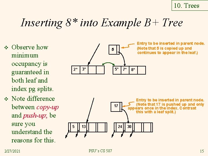
10. Trees Inserting 8* into Example B+ Tree v v Observe how minimum occupancy is guaranteed in both leaf and index pg splits. Note difference between copy-up and push-up; be sure you understand the reasons for this. 2/27/2021 Entry to be inserted in parent node. (Note that 5 is s copied up and continues to appear in the leaf. ) 5 2* 3* 5* 17 5 13 24 PSU’s CS 587 7* 8* Entry to be inserted in parent node. (Note that 17 is pushed up and only appears once in the index. Contrast this with a leaf split. ) 30 15

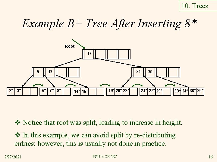
10. Trees Example B+ Tree After Inserting 8* Root 17 5 2* 3* 24 13 5* 7* 8* 14* 16* 19* 20* 22* 30 24* 27* 29* 33* 34* 38* 39* v Notice that root was split, leading to increase in height. v In this example, we can avoid split by re-distributing entries; however, this is usually not done in practice. 2/27/2021 PSU’s CS 587 16

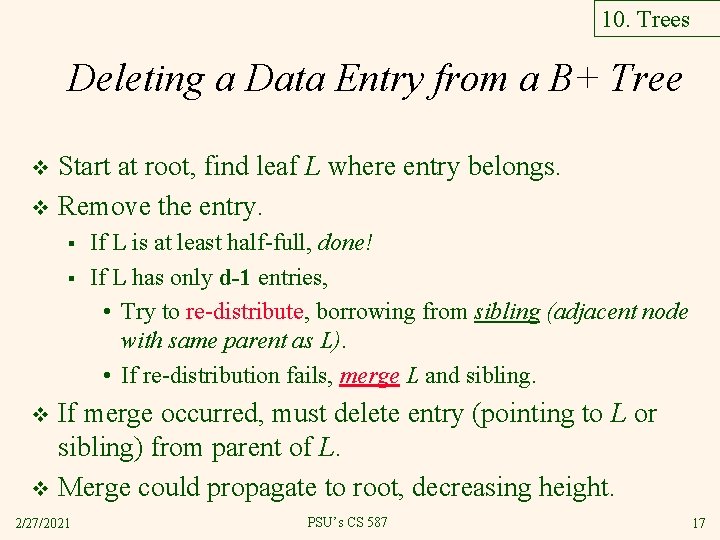
10. Trees Deleting a Data Entry from a B+ Tree Start at root, find leaf L where entry belongs. v Remove the entry. v § § If L is at least half-full, done! If L has only d-1 entries, • Try to re-distribute, borrowing from sibling (adjacent node with same parent as L). • If re-distribution fails, merge L and sibling. If merge occurred, must delete entry (pointing to L or sibling) from parent of L. v Merge could propagate to root, decreasing height. v 2/27/2021 PSU’s CS 587 17

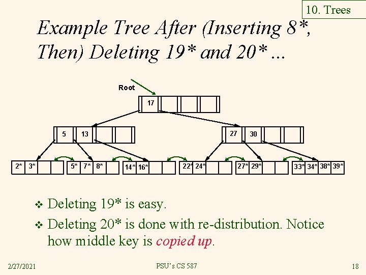
10. Trees Example Tree After (Inserting 8*, Then) Deleting 19* and 20*. . . Root 17 5 2* 3* 27 13 5* 7* 8* 14* 16* 22* 24* 30 27* 29* 33* 34* 38* 39* Deleting 19* is easy. v Deleting 20* is done with re-distribution. Notice how middle key is copied up. v 2/27/2021 PSU’s CS 587 18

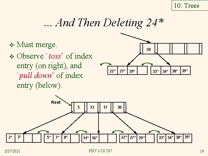
10. Trees . . . And Then Deleting 24* Must merge. v Observe `toss’ of index entry (on right), and `pull down’ of index entry (below). v 30 22* 27* 29* 33* 34* 38* 39* Root 5 2* 3* 2/27/2021 5* 7* 8* 13 17 14* 16* PSU’s CS 587 30 22* 27* 29* 33* 34* 38* 39* 19

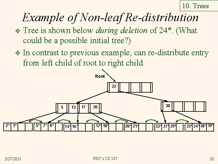
10. Trees Example of Non-leaf Re-distribution Tree is shown below during deletion of 24*. (What could be a possible initial tree? ) v In contrast to previous example, can re-distribute entry from left child of root to right child. v Root 22 5 2* 3* 2/27/2021 5* 7* 8* 13 14* 16* 17 30 20 17* 18* PSU’s CS 587 20* 21* 22* 27* 29* 33* 34* 38* 39* 20

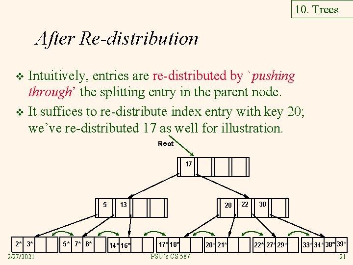
10. Trees After Re-distribution Intuitively, entries are re-distributed by `pushing through’ the splitting entry in the parent node. v It suffices to re-distribute index entry with key 20; we’ve re-distributed 17 as well for illustration. v Root 17 5 2* 3* 2/27/2021 5* 7* 8* 13 14* 16* 20 17* 18* PSU’s CS 587 20* 21* 22 30 22* 27* 29* 33* 34* 38* 39* 21

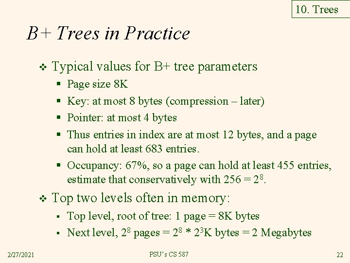
10. Trees B+ Trees in Practice v Typical values for B+ tree parameters § § Page size 8 K Key: at most 8 bytes (compression – later) Pointer: at most 4 bytes Thus entries in index are at most 12 bytes, and a page can hold at least 683 entries. § Occupancy: 67%, so a page can hold at least 455 entries, estimate that conservatively with 256 = 28. v Top two levels often in memory: § § 2/27/2021 Top level, root of tree: 1 page = 8 K bytes Next level, 28 pages = 28 * 23 K bytes = 2 Megabytes PSU’s CS 587 22

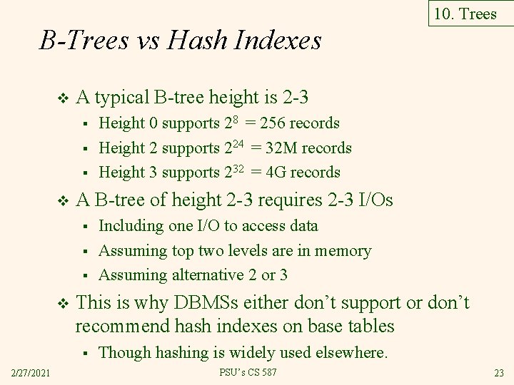
10. Trees B-Trees vs Hash Indexes v A typical B-tree height is 2 -3 § § § v A B-tree of height 2 -3 requires 2 -3 I/Os § § § v Including one I/O to access data Assuming top two levels are in memory Assuming alternative 2 or 3 This is why DBMSs either don’t support or don’t recommend hash indexes on base tables § 2/27/2021 Height 0 supports 28 = 256 records Height 2 supports 224 = 32 M records Height 3 supports 232 = 4 G records Though hashing is widely used elsewhere. PSU’s CS 587 23

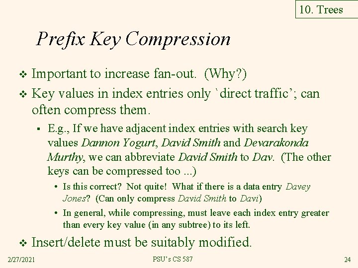
10. Trees Prefix Key Compression Important to increase fan-out. (Why? ) v Key values in index entries only `direct traffic’; can often compress them. v § E. g. , If we have adjacent index entries with search key values Dannon Yogurt, David Smith and Devarakonda Murthy, we can abbreviate David Smith to Dav. (The other keys can be compressed too. . . ) • Is this correct? Not quite! What if there is a data entry Davey Jones? (Can only compress David Smith to Davi) • In general, while compressing, must leave each index entry greater than every key value (in any subtree) to its left. v Insert/delete must be suitably modified. 2/27/2021 PSU’s CS 587 24

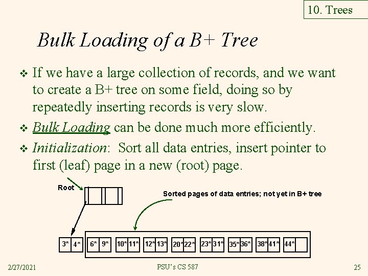
10. Trees Bulk Loading of a B+ Tree If we have a large collection of records, and we want to create a B+ tree on some field, doing so by repeatedly inserting records is very slow. v Bulk Loading can be done much more efficiently. v Initialization: Sort all data entries, insert pointer to first (leaf) page in a new (root) page. v Root 3* 4* 2/27/2021 Sorted pages of data entries; not yet in B+ tree 6* 9* 10* 11* 12* 13* 20* 22* 23* 31* 35* 36* PSU’s CS 587 38* 41* 44* 25

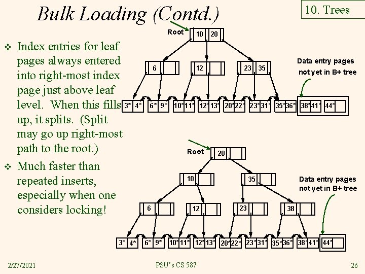
Bulk Loading (Contd. ) Root v v Index entries for leaf pages always entered into right-most index page just above leaf level. When this fills 3* up, it splits. (Split may go up right-most path to the root. ) Much faster than repeated inserts, especially when one considers locking! 6 4* 3* 4* 2/27/2021 10 6* 9* 10. Trees 20 12 23 20 10 12 6* 9* not yet in B+ tree 10* 11* 12* 13* 20*22* 23* 31* 35* 36* 38*41* 44* Root 6 Data entry pages 35 Data entry pages not yet in B+ tree 35 23 38 10* 11* 12* 13* 20*22* 23* 31* 35* 36* 38*41* 44* PSU’s CS 587 26

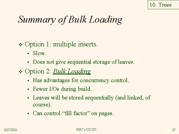
10. Trees Summary of Bulk Loading v Option 1: multiple inserts. § § v Option 2: Bulk Loading § § 2/27/2021 Slow. Does not give sequential storage of leaves. Has advantages for concurrency control. Fewer I/Os during build. Leaves will be stored sequentially (and linked, of course). Can control “fill factor” on pages. PSU’s CS 587 27

10. Trees A Note on `Order’ v Order (d) concept replaced by physical space criterion in practice (`at least half-full’). § § § 2/27/2021 Index pages can typically hold many more entries than leaf pages. Variable sized records and search keys mean different nodes will contain different numbers of entries. Even with fixed length fields, multiple records with the same search key value (duplicates) can lead to variablesized data entries (if we use Alternative (3)). PSU’s CS 587 28

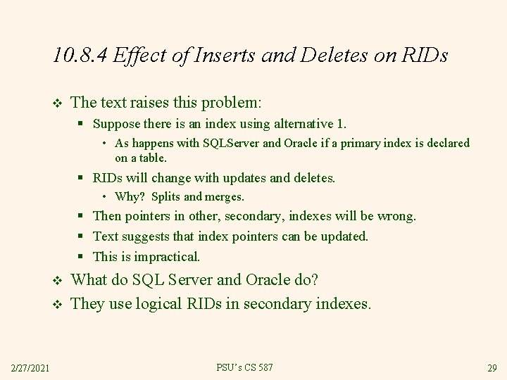
10. 8. 4 Effect of Inserts and Deletes on RIDs v The text raises this problem: § Suppose there is an index using alternative 1. • As happens with SQLServer and Oracle if a primary index is declared on a table. § RIDs will change with updates and deletes. • Why? Splits and merges. § Then pointers in other, secondary, indexes will be wrong. § Text suggests that index pointers can be updated. § This is impractical. v v 2/27/2021 What do SQL Server and Oracle do? They use logical RIDs in secondary indexes. PSU’s CS 587 29

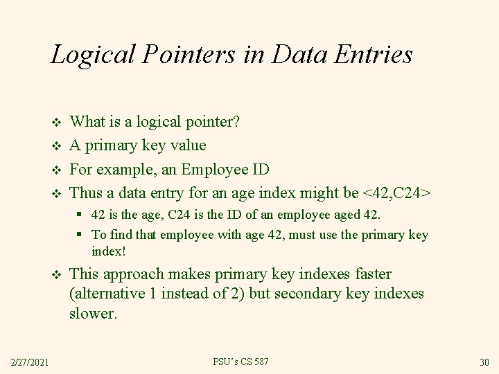
Logical Pointers in Data Entries v v What is a logical pointer? A primary key value For example, an Employee ID Thus a data entry for an age index might be <42, C 24> § 42 is the age, C 24 is the ID of an employee aged 42. § To find that employee with age 42, must use the primary key index! v 2/27/2021 This approach makes primary key indexes faster (alternative 1 instead of 2) but secondary key indexes slower. PSU’s CS 587 30

11. Hash-based Indexes review v As for any index, 3 alternatives for data entries k*: § Data record with key value k § <k, rid of data record with search key value k> § <k, list of rids of data records with search key k> § Choice orthogonal to the indexing technique Hash-based indexes are best for equality selections. Cannot support range searches. v Static and dynamic hashing techniques exist; trade-offs similar to ISAM vs. B+ trees. v 2/27/2021 PSU’s CS 587 31

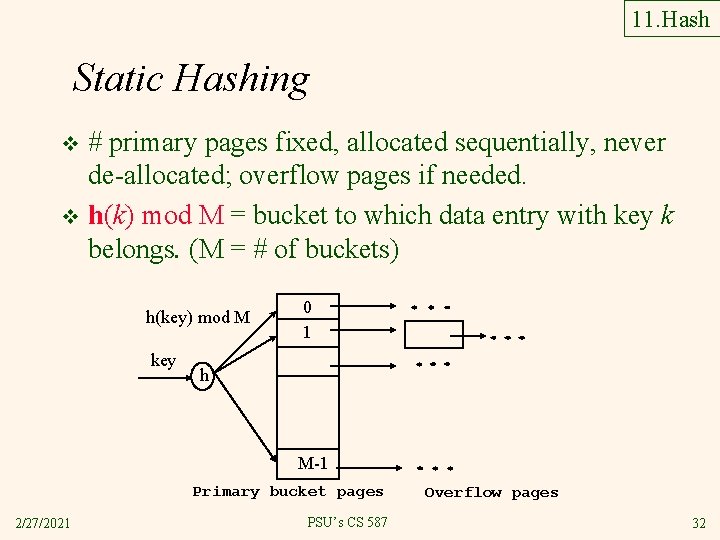
11. Hash Static Hashing # primary pages fixed, allocated sequentially, never de-allocated; overflow pages if needed. v h(k) mod M = bucket to which data entry with key k belongs. (M = # of buckets) v h(key) mod M key 0 1 h M-1 Primary bucket pages 2/27/2021 PSU’s CS 587 Overflow pages 32

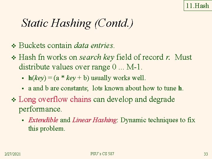
11. Hash Static Hashing (Contd. ) Buckets contain data entries. v Hash fn works on search key field of record r. Must distribute values over range 0. . . M-1. v § § v h(key) = (a * key + b) usually works well. a and b are constants; lots known about how to tune h. Long overflow chains can develop and degrade performance. § 2/27/2021 Extendible and Linear Hashing: Dynamic techniques to fix this problem. PSU’s CS 587 33

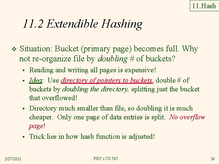
11. Hash 11. 2 Extendible Hashing v Situation: Bucket (primary page) becomes full. Why not re-organize file by doubling # of buckets? § § 2/27/2021 Reading and writing all pages is expensive! Idea: Use directory of pointers to buckets, double # of buckets by doubling the directory, splitting just the bucket that overflowed! Directory much smaller than file, so doubling it is much cheaper. Only one page of data entries is split. No overflow page! Trick lies in how hash function is adjusted! PSU’s CS 587 34

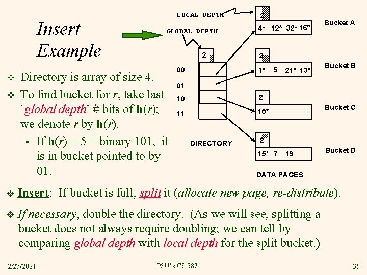
Insert Example v v LOCAL DEPTH GLOBAL DEPTH 2 Directory is array of size 4. To find bucket for r, take last `global depth’ # bits of h(r); we denote r by h(r). § If h(r) = 5 = binary 101, it is in bucket pointed to by 01. 00 2 4* 12* 32* 16* Bucket A 2 1* 5* 21* 13* Bucket B 01 10 2 11 10* DIRECTORY Bucket C 2 15* 7* 19* Bucket D DATA PAGES v Insert: If bucket is full, split it (allocate new page, re-distribute). v If necessary, double the directory. (As we will see, splitting a bucket does not always require doubling; we can tell by comparing global depth with local depth for the split bucket. ) 2/27/2021 PSU’s CS 587 35

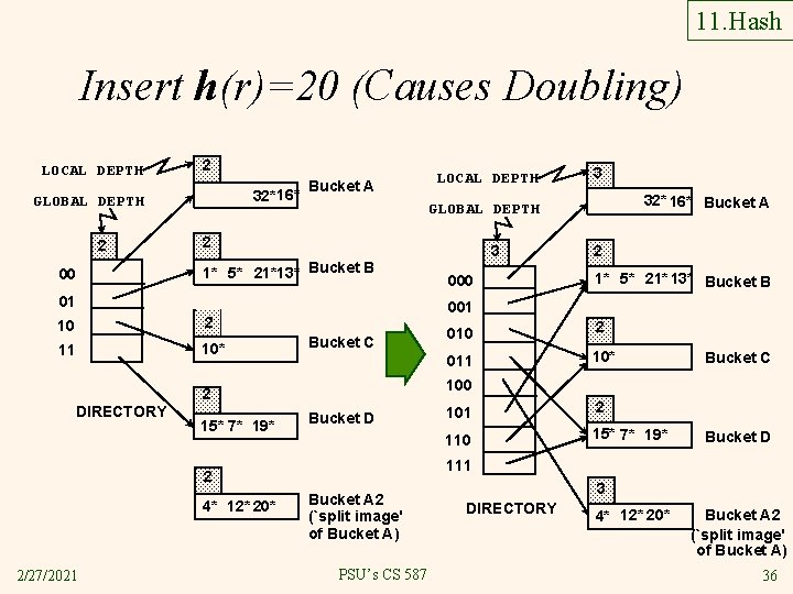
11. Hash Insert h(r)=20 (Causes Doubling) LOCAL DEPTH 2 32*16* GLOBAL DEPTH 2 00 Bucket A 2 1* 5* 21*13* Bucket B 10 2 11 10* Bucket C 2/27/2021 3 000 2 1* 5* 21* 13* Bucket B 010 2 011 10* Bucket C 100 Bucket D 101 2 110 15* 7* 19* Bucket D 111 2 4* 12* 20* 32* 16* Bucket A 001 2 15* 7* 19* 3 GLOBAL DEPTH 01 DIRECTORY LOCAL DEPTH Bucket A 2 (`split image' of Bucket A) PSU’s CS 587 3 DIRECTORY 4* 12* 20* Bucket A 2 (`split image' of Bucket A) 36

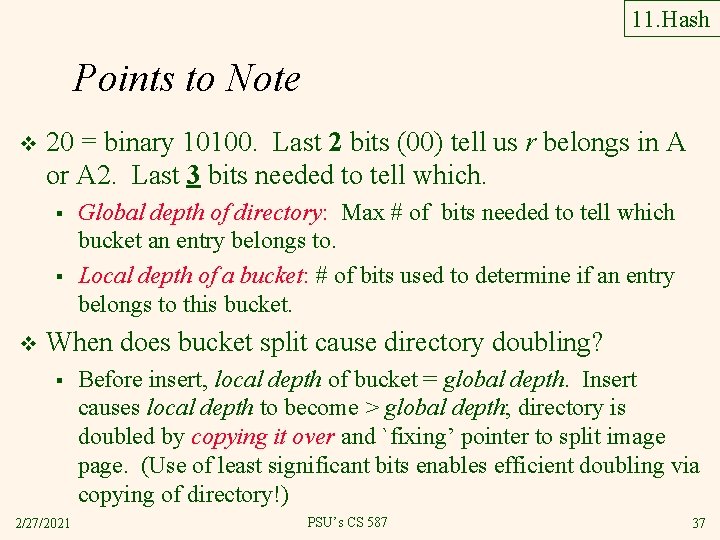
11. Hash Points to Note v 20 = binary 10100. Last 2 bits (00) tell us r belongs in A or A 2. Last 3 bits needed to tell which. § § v Global depth of directory: Max # of bits needed to tell which bucket an entry belongs to. Local depth of a bucket: # of bits used to determine if an entry belongs to this bucket. When does bucket split cause directory doubling? § 2/27/2021 Before insert, local depth of bucket = global depth. Insert causes local depth to become > global depth; directory is doubled by copying it over and `fixing’ pointer to split image page. (Use of least significant bits enables efficient doubling via copying of directory!) PSU’s CS 587 37

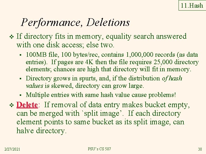
11. Hash Performance, Deletions v If directory fits in memory, equality search answered with one disk access; else two. § § § v 100 MB file, 100 bytes/rec, contains 1, 000 records (as data entries). If pages are 4 K then the file requires 25, 000 directory elements; chances are high that directory will fit in memory. Directory grows in spurts, and, if the distribution of hash values is skewed, directory can grow large. Multiple entries with same hash value cause problems! Delete: If removal of data entry makes bucket empty, can be merged with `split image’. If each directory element points to same bucket as its split image, can halve directory. 2/27/2021 PSU’s CS 587 38

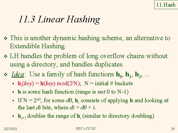
11. Hash 11. 3 Linear Hashing This is another dynamic hashing scheme, an alternative to Extendible Hashing. v LH handles the problem of long overflow chains without using a directory, and handles duplicates. v Idea: Use a family of hash functions h 0, h 1, h 2, . . . v § § 2/27/2021 hi(key) = h(key) mod(2 i. N); N = initial # buckets h is some hash function (range is not 0 to N-1) If N = 2 d 0, for some d 0, hi consists of applying h and looking at the last di bits, where di = d 0 + i. hi+1 doubles the range of hi (similar to directory doubling) PSU’s CS 587 39

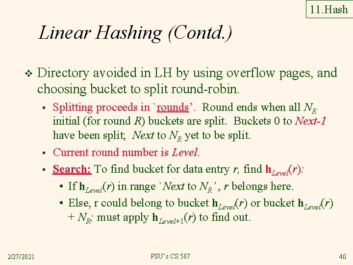
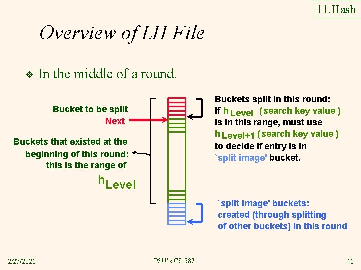
11. Hash Linear Hashing (Contd. ) v Directory avoided in LH by using overflow pages, and choosing bucket to split round-robin. § § § 2/27/2021 Splitting proceeds in `rounds’. Round ends when all NR initial (for round R) buckets are split. Buckets 0 to Next-1 have been split; Next to NR yet to be split. Current round number is Level. Search: To find bucket for data entry r, find h. Level(r): • If h. Level(r) in range `Next to NR’ , r belongs here. • Else, r could belong to bucket h. Level(r) or bucket h. Level(r) + NR; must apply h. Level+1(r) to find out. PSU’s CS 587 40

11. Hash Overview of LH File v In the middle of a round. Buckets split in this round: If h Level ( search key value ) is in this range, must use h Level+1 ( search key value ) to decide if entry is in `split image' bucket. Bucket to be split Next Buckets that existed at the beginning of this round: this is the range of h. Level `split image' buckets: created (through splitting of other buckets) in this round 2/27/2021 PSU’s CS 587 41

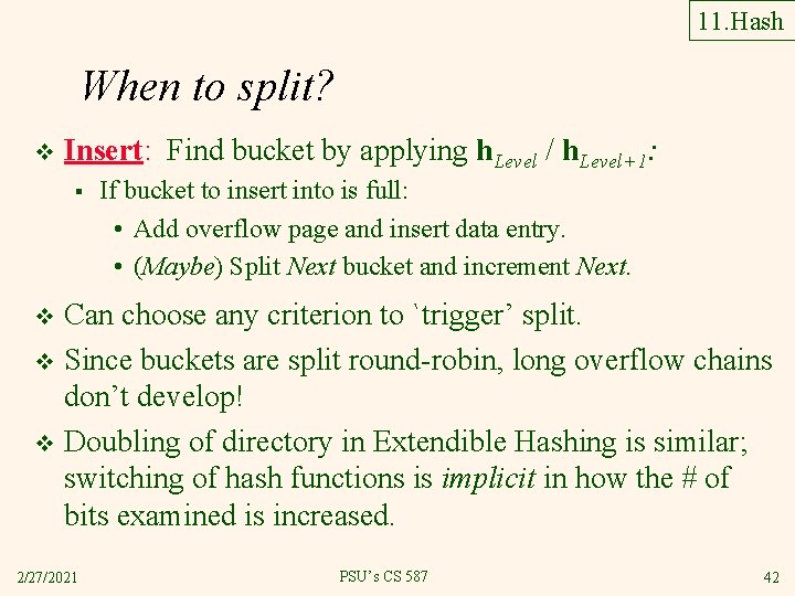
11. Hash When to split? v Insert: Find bucket by applying h. Level / h. Level+1: § If bucket to insert into is full: • Add overflow page and insert data entry. • (Maybe) Split Next bucket and increment Next. Can choose any criterion to `trigger’ split. v Since buckets are split round-robin, long overflow chains don’t develop! v Doubling of directory in Extendible Hashing is similar; switching of hash functions is implicit in how the # of bits examined is increased. v 2/27/2021 PSU’s CS 587 42

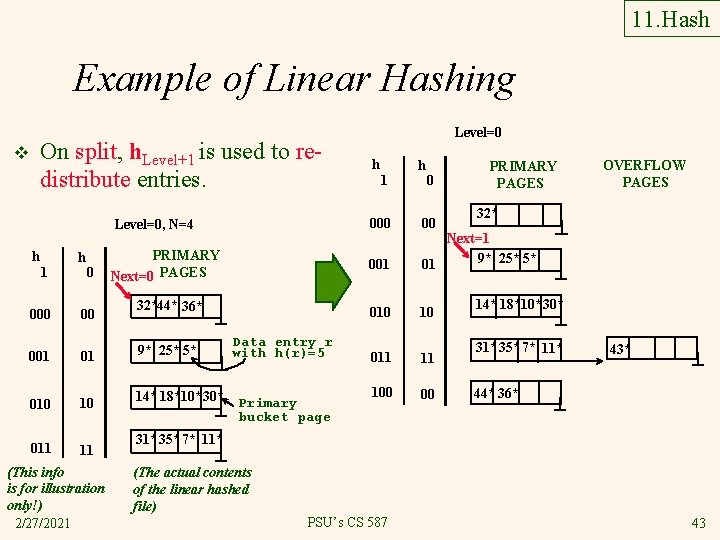
11. Hash Example of Linear Hashing On split, h. Level+1 is used to redistribute entries. v h 1 000 h 0 00 001 01 010 10 011 11 (This info is for illustration only!) 2/27/2021 Level=0 h 1 h 0 PRIMARY PAGES 32* Level=0, N=4 000 00 PRIMARY Next=0 PAGES 001 Next=1 9* 25* 5* 01 010 10 011 11 100 00 32*44* 36* 9* 25* 5* 14* 18*10*30* Data entry r with h(r)=5 Primary bucket page OVERFLOW PAGES 14* 18*10*30* 31*35* 7* 11* 43* 44* 36* 31*35* 7* 11* (The actual contents of the linear hashed file) PSU’s CS 587 43

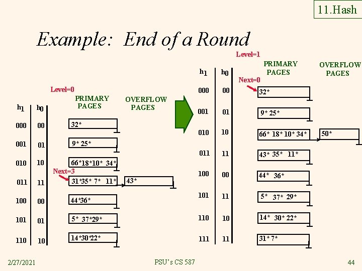
11. Hash Example: End of a Round Level=1 Level=0 h 1 h 0 00 001 010 01 10 PRIMARY PAGES OVERFLOW PAGES 32* PRIMARY PAGES h 1 h 0 00 32* 001 01 9* 25* 010 10 66* 18* 10* 34* 011 11 43* 35* 11* 100 00 44* 36* 101 11 5* 37* 29* Next=0 50* 9* 25* 66*18* 10* 34* Next=3 31*35* 7* 11* 43* 011 11 100 00 44*36* 101 01 5* 37*29* 110 10 14* 30* 22* 110 10 14*30*22* 111 11 31* 7* 2/27/2021 OVERFLOW PAGES PSU’s CS 587 44

11. Hash LH Described as a Variant of EH v The two schemes are actually quite similar: § § § Begin with an EH index where directory has N elements. Use overflow pages, split buckets round-robin. First split is at bucket 0. (Imagine directory being doubled at this point. ) But elements <1, N+1>, <2, N+2>, . . . are the same. So, need only create directory element N, which differs from 0, now. • When bucket 1 splits, create directory element N+1, etc. v So, directory can double gradually. Also, primary bucket pages are created in order. If they are allocated in sequence too (so that finding i’th is easy), we actually don’t need a directory! Voila, LH. 2/27/2021 PSU’s CS 587 45