Chapter 1 Section 1 Solving Linear Equations in

Chapter 1 – Section 1 Solving Linear Equations in One Variable

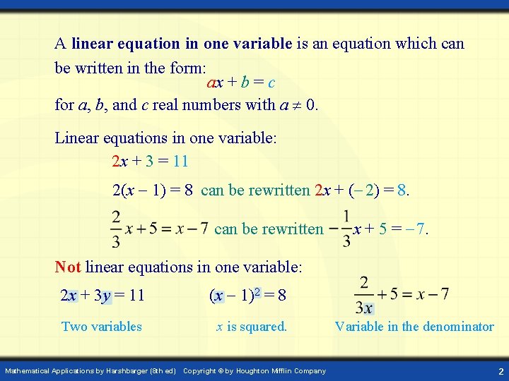
A linear equation in one variable is an equation which can be written in the form: ax + b = c for a, b, and c real numbers with a 0. Linear equations in one variable: 2 x + 3 = 11 2(x 1) = 8 can be rewritten 2 x + ( 2) = 8. can be rewritten x + 5 = 7. Not linear equations in one variable: 2 x + 3 y = 11 (x 1)2 = 8 Two variables x is squared. Mathematical Applications by Harshbarger (8 th ed) Copyright © by Houghton Mifflin Company Variable in the denominator 2

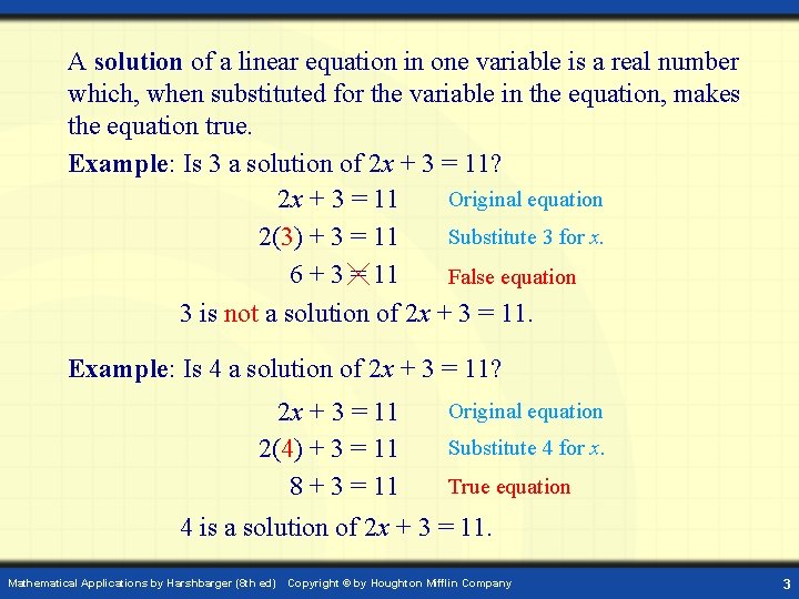
A solution of a linear equation in one variable is a real number which, when substituted for the variable in the equation, makes the equation true. Example: Is 3 a solution of 2 x + 3 = 11? Original equation 2 x + 3 = 11 Substitute 3 for x. 2(3) + 3 = 11 6 + 3 = 11 False equation 3 is not a solution of 2 x + 3 = 11. Example: Is 4 a solution of 2 x + 3 = 11? 2 x + 3 = 11 2(4) + 3 = 11 8 + 3 = 11 Original equation Substitute 4 for x. True equation 4 is a solution of 2 x + 3 = 11. Mathematical Applications by Harshbarger (8 th ed) Copyright © by Houghton Mifflin Company 3

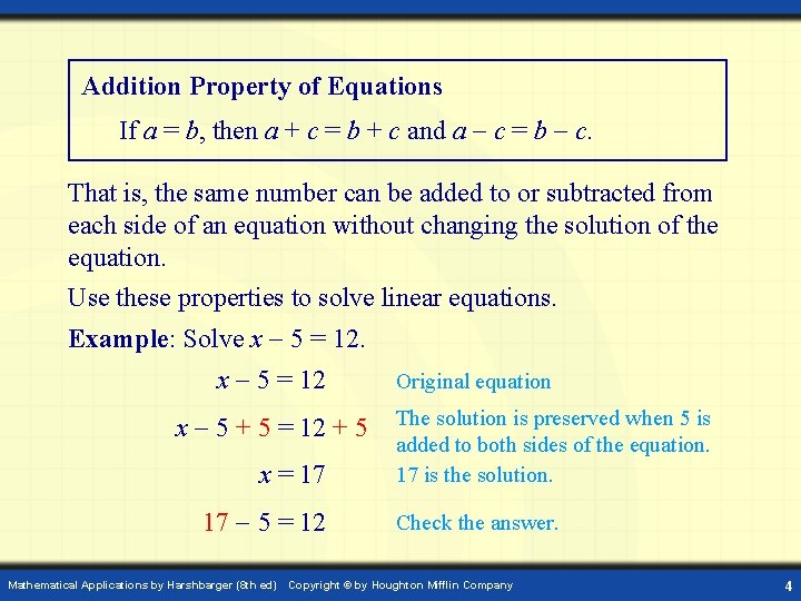
Addition Property of Equations If a = b, then a + c = b + c and a c = b c. That is, the same number can be added to or subtracted from each side of an equation without changing the solution of the equation. Use these properties to solve linear equations. Example: Solve x 5 = 12 x 5 + 5 = 12 + 5 x = 17 17 5 = 12 Mathematical Applications by Harshbarger (8 th ed) Original equation The solution is preserved when 5 is added to both sides of the equation. 17 is the solution. Check the answer. Copyright © by Houghton Mifflin Company 4

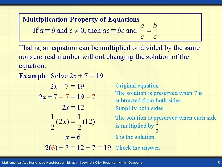
Multiplication Property of Equations If a = b and c 0, then ac = bc and . That is, an equation can be multiplied or divided by the same nonzero real number without changing the solution of the equation. Example: Solve 2 x + 7 = 19. Original equation 2 x + 7 = 19 The solution is preserved when 7 is 2 x + 7 7 = 19 7 subtracted from both sides. 2 x = 12 Simplify both sides. The solution is preserved when each side is multiplied by. 6 is the solution. x=6 2(6) + 7 = 12 + 7 = 19 Check the answer. Mathematical Applications by Harshbarger (8 th ed) Copyright © by Houghton Mifflin Company 5

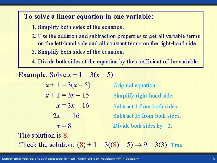
To solve a linear equation in one variable: 1. Simplify both sides of the equation. 2. Use the addition and subtraction properties to get all variable terms on the left-hand side and all constant terms on the right-hand side. 3. Simplify both sides of the equation. 4. Divide both sides of the equation by the coefficient of the variable. Example: Solve x + 1 = 3(x 5) Original equation x + 1 = 3 x 15 Simplify right-hand side. x = 3 x 16 Subtract 1 from both sides. Subtract 3 x from both sides. 2 x = 16 Divide both sides by 2. x=8 The solution is 8. Check the solution: (8) + 1 = 3((8) 5) 9 = 3(3) True Mathematical Applications by Harshbarger (8 th ed) Copyright © by Houghton Mifflin Company 6

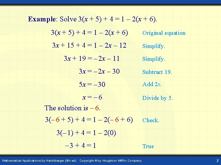
Example: Solve 3(x + 5) + 4 = 1 – 2(x + 6) Original equation 3 x + 15 + 4 = 1 – 2 x – 12 Simplify. 3 x + 19 = – 2 x – 11 Simplify. 3 x = – 2 x – 30 Subtract 19. 5 x = – 30 Add 2 x. x = 6 The solution is 6. Divide by 5. 3(– 6 + 5) + 4 = 1 – 2(– 6 + 6) Check. 3(– 1) + 4 = 1 – 2(0) 3 + 4 = 1 Mathematical Applications by Harshbarger (8 th ed) Copyright © by Houghton Mifflin Company True 7

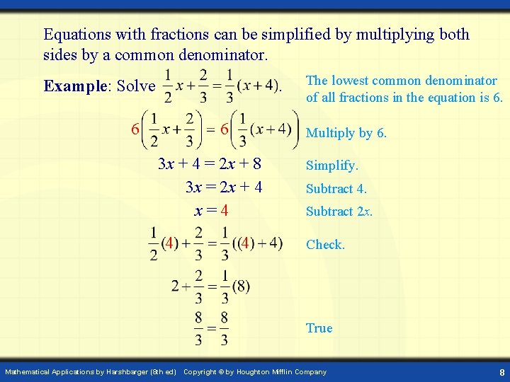
Equations with fractions can be simplified by multiplying both sides by a common denominator. Example: Solve . 6 6 Multiply by 6. 3 x + 4 = 2 x + 8 3 x = 2 x + 4 x=4 4 The lowest common denominator of all fractions in the equation is 6. 4 Simplify. Subtract 4. Subtract 2 x. Check. True Mathematical Applications by Harshbarger (8 th ed) Copyright © by Houghton Mifflin Company 8

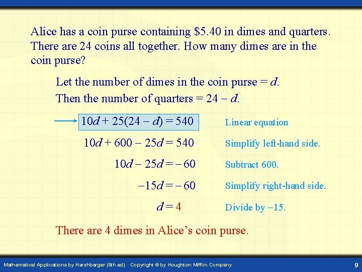
Alice has a coin purse containing $5. 40 in dimes and quarters. There are 24 coins all together. How many dimes are in the coin purse? Let the number of dimes in the coin purse = d. Then the number of quarters = 24 d. 10 d + 25(24 d) = 540 Linear equation 10 d + 600 25 d = 540 Simplify left-hand side. 10 d 25 d = 60 15 d = 60 d=4 Subtract 600. Simplify right-hand side. Divide by 15. There are 4 dimes in Alice’s coin purse. Mathematical Applications by Harshbarger (8 th ed) Copyright © by Houghton Mifflin Company 9

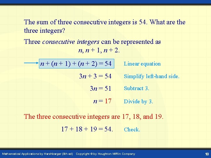
The sum of three consecutive integers is 54. What are three integers? Three consecutive integers can be represented as n, n + 1, n + 2. n + (n + 1) + (n + 2) = 54 3 n + 3 = 54 3 n = 51 n = 17 Linear equation Simplify left-hand side. Subtract 3. Divide by 3. The three consecutive integers are 17, 18, and 19. 17 + 18 + 19 = 54. Mathematical Applications by Harshbarger (8 th ed) Check. Copyright © by Houghton Mifflin Company 10

Digital Lesson Linear Equations in Two Variables

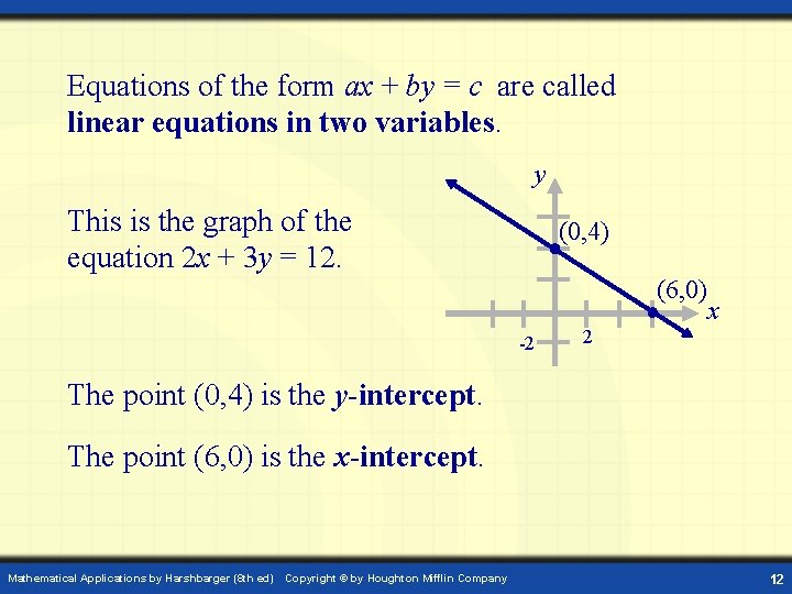
Equations of the form ax + by = c are called linear equations in two variables. y This is the graph of the equation 2 x + 3 y = 12. (0, 4) (6, 0) -2 x 2 The point (0, 4) is the y-intercept. The point (6, 0) is the x-intercept. Mathematical Applications by Harshbarger (8 th ed) Copyright © by Houghton Mifflin Company 12

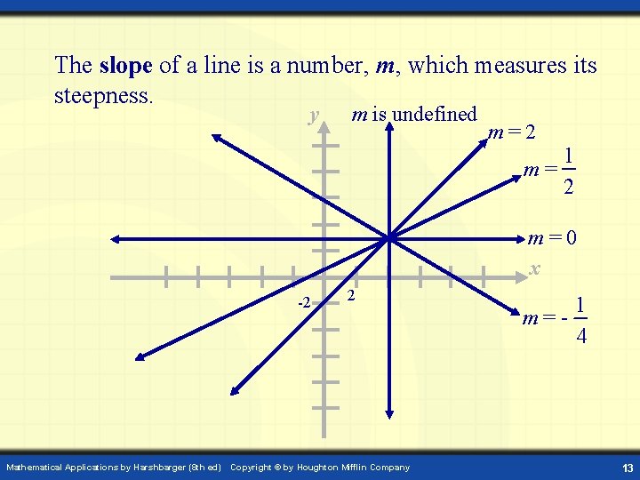
The slope of a line is a number, m, which measures its steepness. y m is undefined m=2 1 m= 2 m=0 x -2 Mathematical Applications by Harshbarger (8 th ed) 2 Copyright © by Houghton Mifflin Company 1 m=4 13

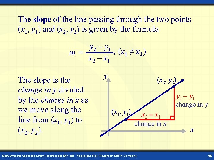
The slope of the line passing through the two points (x 1, y 1) and (x 2, y 2) is given by the formula y 2 – y 1 , (x 1 ≠ x 2 ). m= x 2 – x 1 The slope is the change in y divided by the change in x as we move along the line from (x 1, y 1) to (x 2, y 2). Mathematical Applications by Harshbarger (8 th ed) y (x 2, y 2) (x 1, y 1) y 2 – y 1 change in y x 2 – x 1 change in x Copyright © by Houghton Mifflin Company x 14

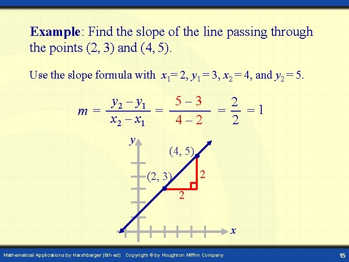
Example: Find the slope of the line passing through the points (2, 3) and (4, 5). Use the slope formula with x 1= 2, y 1 = 3, x 2 = 4, and y 2 = 5. y 2 – y 1 5– 3 m= = x 2 – x 1 4– 2 y 2 = =1 2 (4, 5) 2 (2, 3) 2 x Mathematical Applications by Harshbarger (8 th ed) Copyright © by Houghton Mifflin Company 15

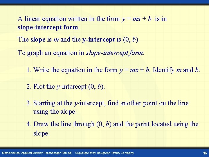
A linear equation written in the form y = mx + b is in slope-intercept form. The slope is m and the y-intercept is (0, b). To graph an equation in slope-intercept form: 1. Write the equation in the form y = mx + b. Identify m and b. 2. Plot the y-intercept (0, b). 3. Starting at the y-intercept, find another point on the line using the slope. 4. Draw the line through (0, b) and the point located using the slope. Mathematical Applications by Harshbarger (8 th ed) Copyright © by Houghton Mifflin Company 16

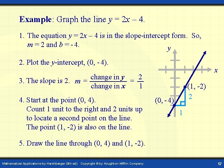
Example: Graph the line y = 2 x – 4. 1. The equation y = 2 x – 4 is in the slope-intercept form. So, m = 2 and b = - 4. y 2. Plot the y-intercept, (0, - 4). x 3. The slope is 2. m = change in y = 2 1 change in x 4. Start at the point (0, 4). Count 1 unit to the right and 2 units up to locate a second point on the line. The point (1, -2) is also on the line. (1, -2) 2 (0, - 4) 1 5. Draw the line through (0, 4) and (1, -2). Mathematical Applications by Harshbarger (8 th ed) Copyright © by Houghton Mifflin Company 17

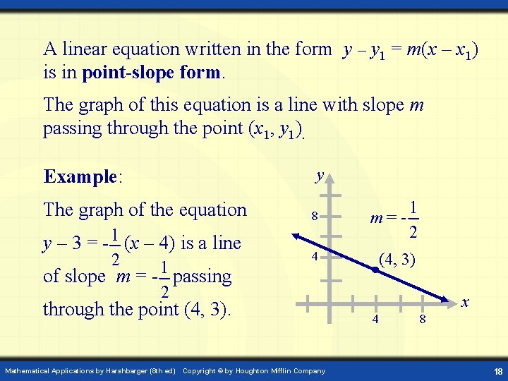
A linear equation written in the form y – y 1 = m(x – x 1) is in point-slope form. The graph of this equation is a line with slope m passing through the point (x 1, y 1). y Example: The graph of the equation y – 3 = - 1 (x – 4) is a line 2 of slope m = - 1 passing 2 8 4 through the point (4, 3). Mathematical Applications by Harshbarger (8 th ed) m=- Copyright © by Houghton Mifflin Company 1 2 (4, 3) x 4 8 18

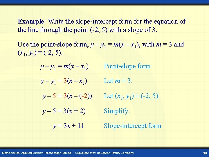
Example: Write the slope-intercept form for the equation of the line through the point (-2, 5) with a slope of 3. Use the point-slope form, y – y 1 = m(x – x 1), with m = 3 and (x 1, y 1) = (-2, 5). y – y 1 = m(x – x 1) Point-slope form y – y 1 = 3(x – x 1) Let m = 3. y – 5 = 3(x – (-2)) Let (x 1, y 1) = (-2, 5). y – 5 = 3(x + 2) Simplify. y = 3 x + 11 Mathematical Applications by Harshbarger (8 th ed) Slope-intercept form Copyright © by Houghton Mifflin Company 19

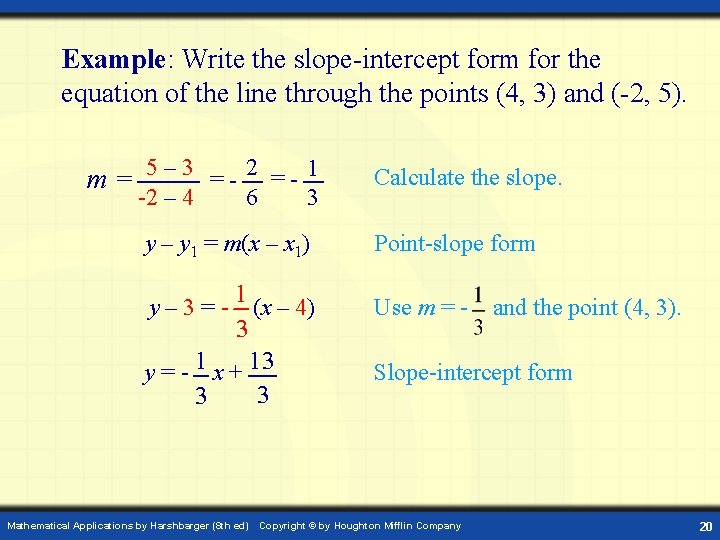
Example: Write the slope-intercept form for the equation of the line through the points (4, 3) and (-2, 5). 5– 3 =- 2 =- 1 m= -2 – 4 6 3 y – y 1 = m(x – x 1) 1 (x – 4) 3 y = - 1 x + 13 3 3 y– 3=- Mathematical Applications by Harshbarger (8 th ed) Calculate the slope. Point-slope form Use m = - and the point (4, 3). Slope-intercept form Copyright © by Houghton Mifflin Company 20

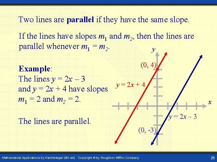
Two lines are parallel if they have the same slope. If the lines have slopes m 1 and m 2, then the lines are parallel whenever m 1 = m 2. y (0, 4) Example: The lines y = 2 x – 3 y = 2 x + 4 and y = 2 x + 4 have slopes m 1 = 2 and m 2 = 2. The lines are parallel. Mathematical Applications by Harshbarger (8 th ed) x y = 2 x – 3 (0, -3) Copyright © by Houghton Mifflin Company 21

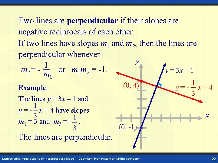
Two lines are perpendicular if their slopes are negative reciprocals of each other. If two lines have slopes m 1 and m 2, then the lines are perpendicular whenever y 1 m 2= or m 1 m 2 = -1. y = 3 x – 1 m 1 (0, 4) Example: The lines y = 3 x – 1 and 1 y = - x + 4 have slopes 3 1 m 1 = 3 and m 2 = -. 3 1 y=- x+4 3 x (0, -1) The lines are perpendicular. Mathematical Applications by Harshbarger (8 th ed) Copyright © by Houghton Mifflin Company 22