Chapter 1 Ray Optics Postulates of Ray Optics

Chapter 1. Ray Optics

Postulates of Ray Optics ds A B

Reflection and Refraction

Fermat’s Principle: Law of Reflection Fermat’s principle: Light rays will travel from point A to point B in a medium along a path that minimizes the time of propagation. B (x 3, y 3) qr (0, y 2) qi y A (x 1, y 1) x : Law of reflection

Fermat’s Principle: Law of Refraction Law of refraction: (x 1, y 1) A y qi x (x 2, 0) ni nt qt (x 3, y 3) : Law of refraction in paraxial approx.

Refraction –Snell’s Law :

Negative index of refraction : n < 0 RHM N>1 N = -1 LHM

Principle of reversibility

Coherent perfect absorbers(CPA): time-reversibility Time-reversed lasers, Lasing in reverse, Suckers for light silicon Time-reversed lasing and interferometric control of absorption, Science , vol. 331, 889 (2011. 2. 18)

Reflection in plane mirrors

Plane surface – Image formation

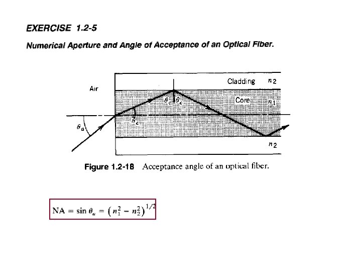
Total internal Reflection (TIR)

Imaging by an Optical System

Cartesian Surfaces • A Cartesian surface – those which form perfect images of a point object • E. g. ellipsoid and hyperboloid O I

Imaging by Cartesian reflecting surfaces

Imaging by Cartesian refracting Surfaces

Approximation by Spherical Surfaces

Reflection at a Spherical Surface

Reflection at Spherical Surfaces I Reflection from a spherical convex surface gives rise to a virtual image. Rays appear to emanate from point I behind the spherical reflector. Use paraxial or small-angle approximation for analysis of optical systems:

Reflection at Spherical Surfaces II Considering Triangle OPC and then Triangle OPI we obtain: Combining these relations we obtain: Again using the small angle approximation:

Reflection at Spherical Surfaces III Image distance s' in terms of the object distance s and mirror radius R: At this point the sign convention in the book is changed ! The following sign convention must be followed in using this equation: 1. Assume that light propagates from left to right. Object distance s is positive when point O is to the left of point V. 2. Image distance s' is positive when I is to the left of V (real image) and negative when to the right of V (virtual image). 3. Mirror radius of curvature R is positive for C to the right of V (convex), negative for C to left of V (concave).

Reflection at Spherical Surfaces IV R<0 f >0 R>0 f <0 The focal length f of the spherical mirror surface is defined as –R/2, where R is the radius of curvature of the mirror. In accordance with the sign convention of the previous page, f > 0 for a concave mirror and f < 0 for a convex mirror. The imaging equation for the spherical mirror can be rewritten as

Reflection at Spherical Surfaces VII Real, Inverted Image Virtual Image, Not Inverted

Refraction

Prisms

Beamsplitters

Spherical boundaries and lenses At point P we apply the law of refraction to obtain Using the small angle approximation we obtain Substituting for the angles q 1 and q 2 we obtain Neglecting the distance QV and writing tangents for the angles gives n 2 > n 1

Refraction by Spherical Surfaces Rearranging the equation we obtain Using the same sign convention as for mirrors we obtain P : power of the refracting surface n 2 > n 1

Example : Concept of imaging by a lens

Thin (refractive) lenses

The Thin Lens Equation I n 1 n 2 O' C 1 O V 1 C 2 V 2 For surface 1: s 1 t s'1

The Thin Lens Equation II For surface 1: For surface 2: Object for surface 2 is virtual, with s 2 given by: For a thin lens: Substituting this expression we obtain:

The Thin Lens Equation III Simplifying this expression we obtain: For the thin lens: The focal length for the thin lens is found by setting s = ∞:

The Thin Lens Equation IV In terms of the focal length f the thin lens equation becomes: The focal length of a thin lens is positive for a convex lens, negative for a concave lens.

Image Formation by Thin Lenses Convex Lens Concave Lens

Image Formation by Convex Lens, focal length = 5 cm: ho F F RI hi

Image Formation by Concave Lens, focal length = -5 cm: ho hi F VI F

Image Formation: Two-Lens System I 60 cm

Image Formation: Two-Lens System II 7 cm

Image Formation Summary Table

Image Formation Summary Figure

Vergence and refractive power : Diopter D>0 D<0 reciprocals Vergence (V) : curvature of wavefront at the lens Refracting power (P) Diopter (D) : unit of vergence (reciprocal length in meter)

Two more useful equations

2 -12. Cylindrical lenses

Cylindrical lenses Top view Side view

D. Light guides

1 -3. Graded-index (GRIN) optics

Rays in heterogeneous media The optical path length between two points x 1 and x 2 through which a ray passes is Written in terms of parameter s , Because the optical path length integral is an extremum (Fermat principle), the integrand L satisfies the Euler equations. For an arbitrary coordinate system , with coordinates q 1 , q 2 , q 3, Lagrange’s equations

GRIN In Cartesian coordinates so the x equation is Similar equations hold for y and z. In Cartesian Coordinates with Parameter s = s. : Ray equation Paraxial Ray Equation ds ~ dz

GRIN slab : n = n(y) n=n(y) : paraxial ray equation % Derivation of the Paraxial Ray Equation in a Graded-Index Slab Using Snell’s Law The two angles are related by Snell’s law,

Ex. 1. 3 -1 GRIN slab with Assuming an initial position y(0) = yo, dy/dz = qo at z = 0,

GRIN fibers

1. 4 Matrix optics : Ray transfer matrix In the par-axial approximation,

What is the ray-transfer matrix

How to use the ray-transfer matrices

How to use the ray-transfer matrices

Translation Matrix ( y 1, a 1 ) ( y o, a o ) L

Refraction Matrix y=y’

Reflection Matrix y=y’

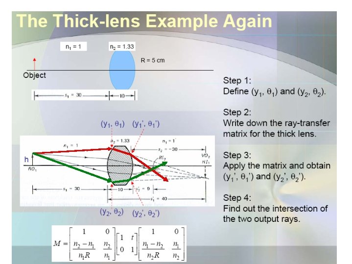
Thick Lens Matrix I

Thick Lens Matrix II

Thin Lens Matrix The thin lens matrix is found by setting t = 0: n. L

Summary of Matrix Methods

Summary of Matrix Methods

System Ray-Transfer Matrix Introduction to Matrix Methods in Optics, A. Gerrard and J. M. Burch

System Ray-Transfer Matrix Any paraxial optical system, no matter how complicated, can be represented by a 2 x 2 optical matrix. This matrix M is usually denoted A useful property of this matrix is that where n 0 and nf are the refractive indices of the initial and final media of the optical system. Usually, the medium will be air on both sides of the optical system and

Significance of system matrix elements The matrix elements of the system matrix can be analyzed to determine the cardinal points and planes of an optical system. Let’s examine the implications when any of the four elements of the system matrix is equal to zero. D=0 : input plane = first focal plane A=0 : output plane = second focal plane B=0 : input and output planes correspond to conjugate planes C=0 : telescopic system

D=0 A=0 B=0 C=0

System Matrix with D=0 Let’s see what happens when D = 0. When D = 0, the input plane for the optical system is the input focal plane.

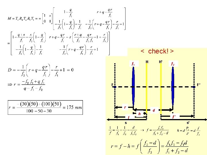
Ex) Two-Lens System f 1 = +50 mm Input Plane F 1 r T 1 f 2 = +30 mm F 2 s q = 100 mm R 1 T 2 Output Plane R 2 T 3

System Matrix with A=0, C=0 When A = 0, the output plane for the optical system is the output focal plane. When C = 0, collimated light at the input plane is collimated light at the exit plane but the angle with the optical axis is different. This is a telescopic arrangement, with a magnification of D = af/a 0.

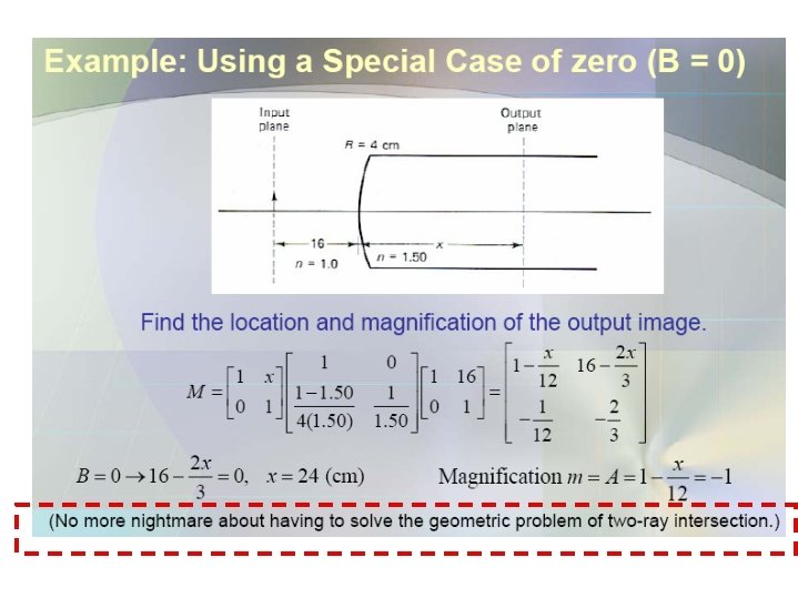
System Matrix with B=0 When B = 0, the input and output planes are object and image planes, respectively, and the transverse magnification of the system m = A.

Ex) Two-Lens System with B=0 f 1 = +50 mm Object Plane F 1 r T 1 f 2 = +30 mm F 2 s q = 100 mm R 1 T 2 Image Plane R 2 T 3