Chapter 1 Probability Basics A Retrospective 1 1

Chapter 1 Probability Basics: A Retrospective 1. 1 What Is "Probability"? 1. 2 The Additive Law 1. 3 Conditional Probability and Independence 1. 4 Permutations and Combinations 1. 5 Continuous Random Variables 1. 6 Countability and Measure Theory 1. 7 Moments 1. 8 Derived Distributions 1. 9 The Normal or Gaussian Distribution 1. 10 Multivariate Statistics 1. 11 Bivariate probability density functions 1. 12 The Bivariate Gaussian Distribution 1. 13 Sums of Random Variables 1. 14 The Multivariate Gaussian

Figure 1. 1 Billiard balls and sky

Figure 1. 2 The Universe of Elemental Events Figure 1. 3 The truth set of statement A
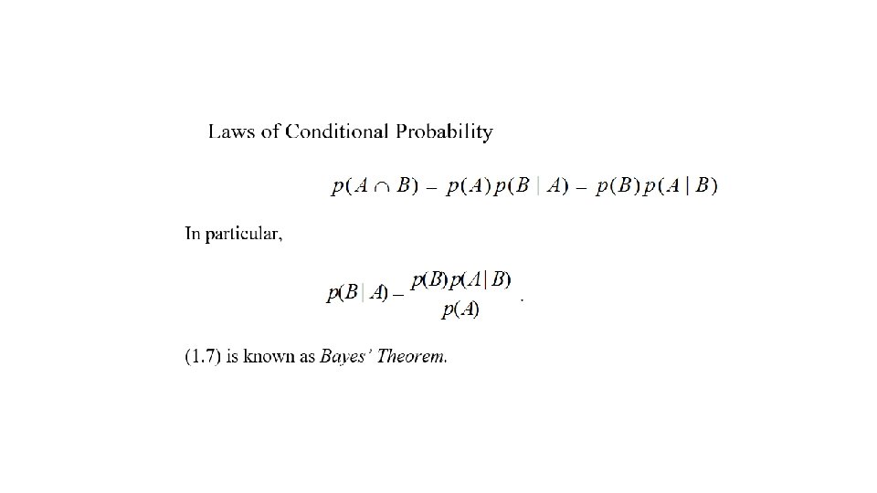
 = p(A) + p(B) - p(A B) Figure 1. 4 Additive Law")
p(A B) = p(A) + p(B) - p(A B) Figure 1. 4 Additive Law of Probability

Figure 1. 5 Universe Figure 1. 6 Conditional universe, given A

Figure 1. 7 a priori Universe Figure 1. 8 Conditional Universe
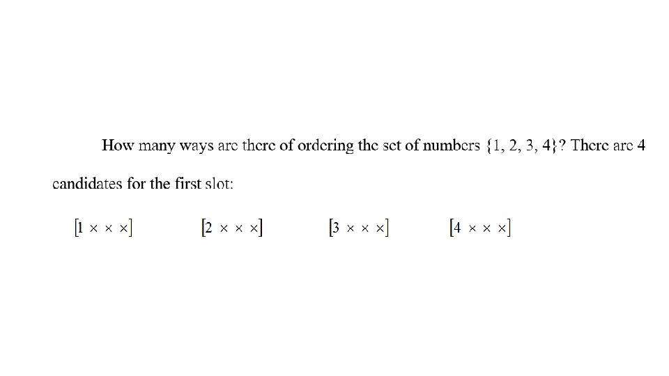
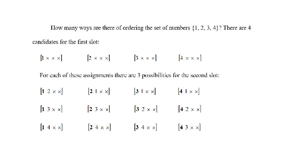
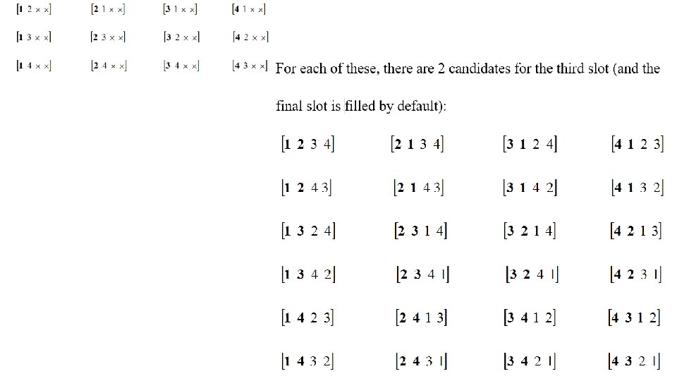

There are 4 3 2 = 4! orderings or permutations of 4 objects.
![The combination [1 3 : 2 4] appears 4 times in the displays of](http://slidetodoc.com/presentation_image_h2/ad589c8363faf6fd3840c45efabe467b/image-14.jpg "The combination [1 3 : 2 4] appears 4 times in the displays of")
The combination [1 3 : 2 4] appears 4 times in the displays of permutations. There are 4!/(2!2!) = 6 ways of selecting the first pair: (1, 2) (1, 3) (1, 4) (2, 3) (2, 4) (3, 4)

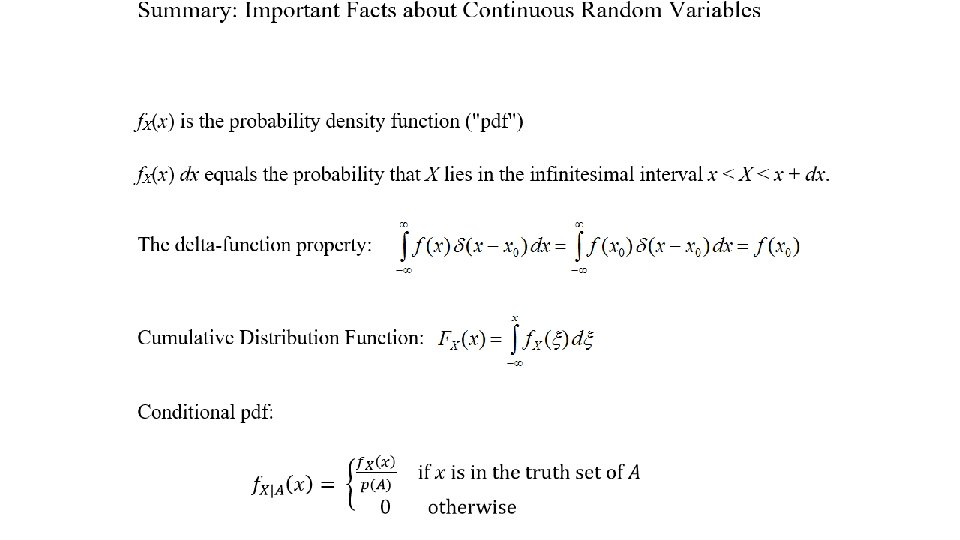
Figure 1. 9 Probability density function

Figure 1. 10 Skewed pdf
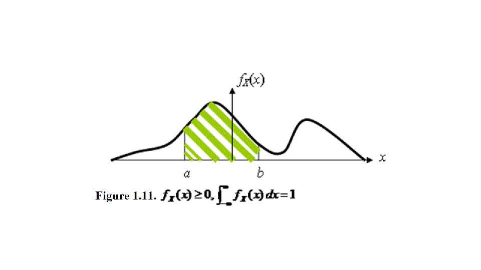

Figure 1. 13 Delta function Figure 1. 12 "Approximate" probability density functions

Figure 1. 14 and 1. 15 Mixed discrete and continuous pdf

Figure 1. 16 Cumulative distribution function
")
Figure 1. 17 Proposed enumeration of (0, 1)
 variable")
Figure 1. 19 Change of (random) variable

Figure 1. 20 Changing variables
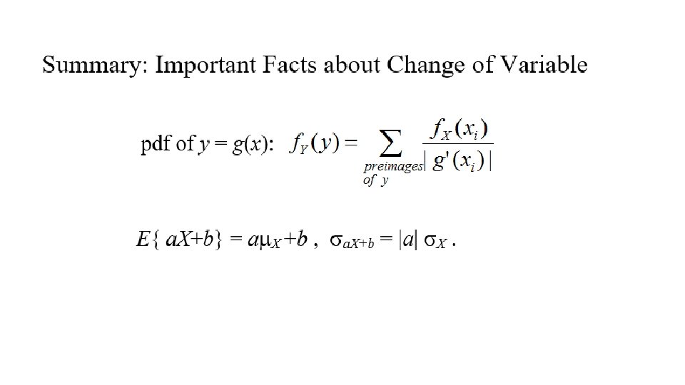

Figure 1. 21 Bell curve

Figure 1. 22 Integration in polar coordinates
")
Figure 1. 23 Normal Distribution N( , )
, N(0, 1), N(0, 0. 2)")
Figure 1. 24 N(0, 2), N(0, 1), N(0, 0. 2)
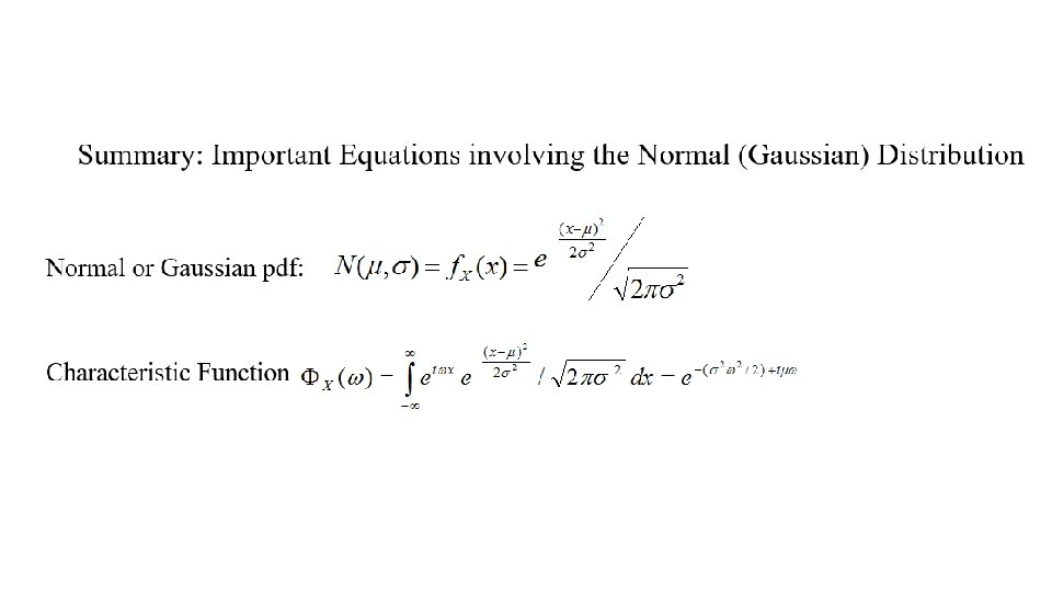

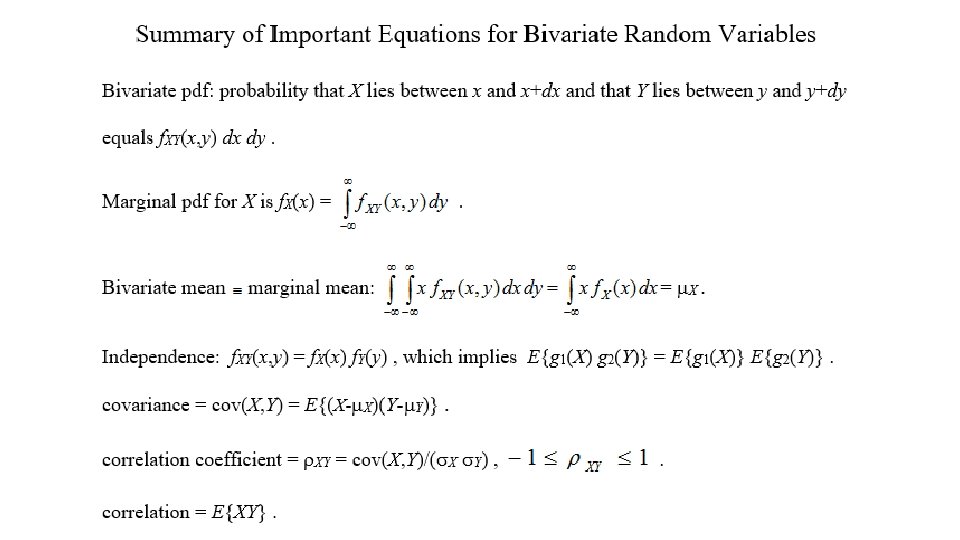
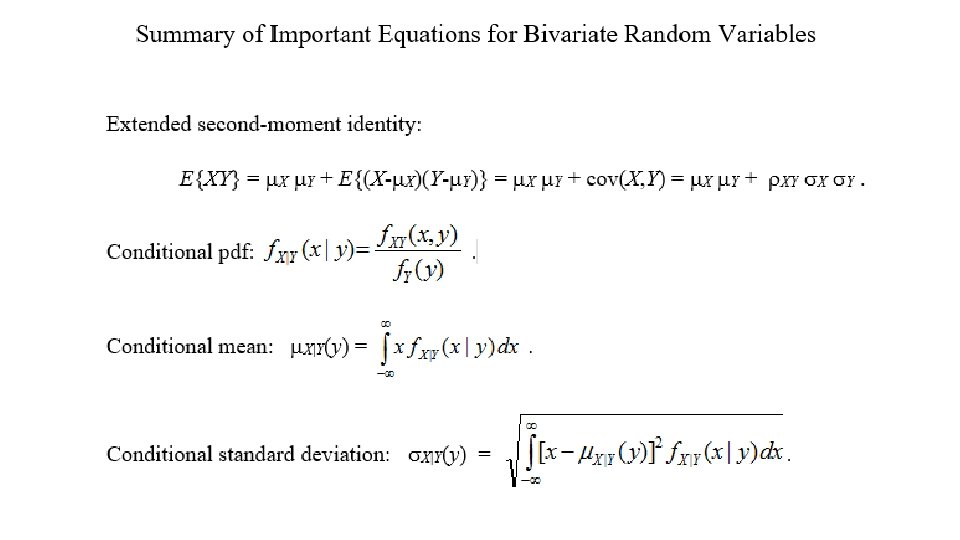
Figure 1. 25 Bivariate pdf element

Figure 1. 26 Marginal probability density

Figure 1. 27, 1. 28 Independent variables Figure 1. 29 Dependent variables

Bivariate Gaussian
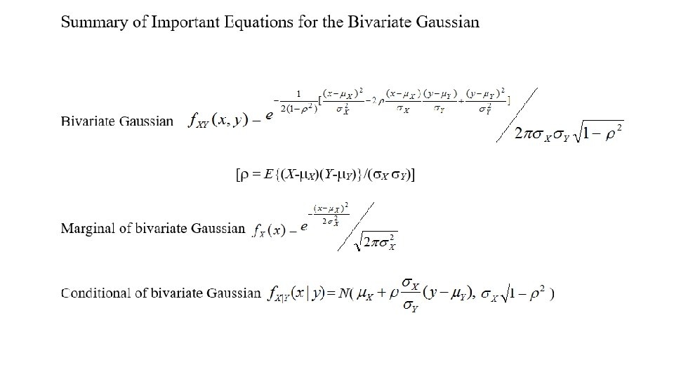
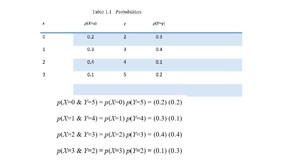
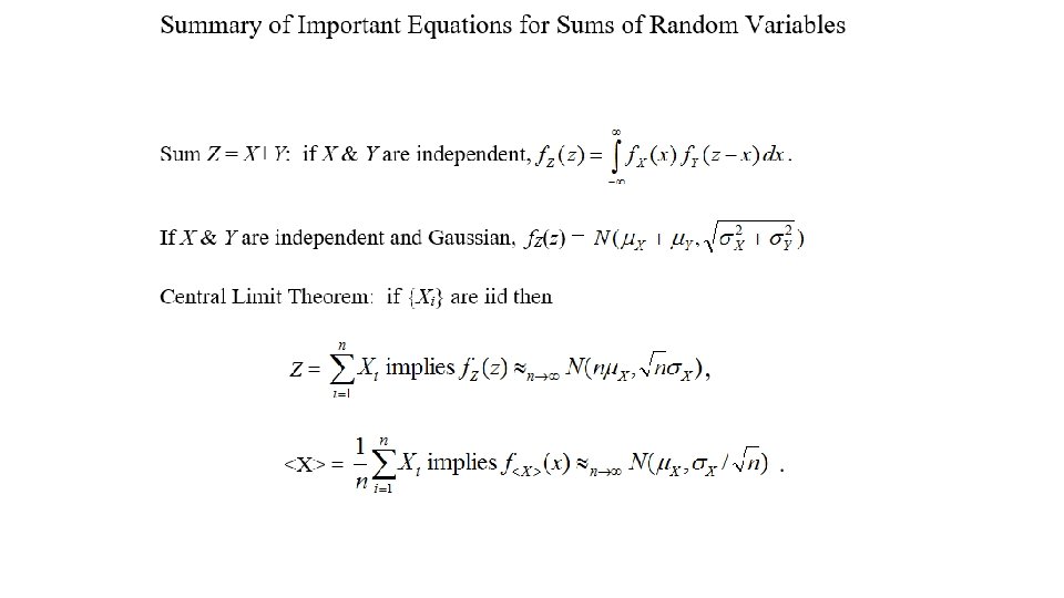

Figure 1. 34 Iterated convolutions Figure 1. 35 Sums of coin flips

The Multivariate Gaussian

Chapter 2 Random Processes 2. 1 Examples of random processes 2. 2 The Mathematical Characterization of Random Processes 2. 3 Prediction: The Statistician's Task

Figure 2. 1 Stock market samples

Figure 2. 2 3 -year temperature chart

Figure 2. 3 Johnson noise

Figure 2. 4 Shot noise

Figure 2. 5 Popcorn noise

Figure 2. 6 ARMA simulation

Figure 2. 7 Bernoulli Process

Figure 2. 8 Random Settings for a DC Power Supply

Figure 2. 9 Random Settings for an AC Power Supply

Figure 2. 10 AC Power Supply Voltages with Random Phase

Figure 2. 11 Continuous, Discrete, and Deterministic pdf's for a Random Process
 at different times")
Figure 2. 12 pdf's for X(t) at different times
(x) for the Bernoulli Process")
Figure 2. 13 f. X(t)(x) for the Bernoulli Process
 = 1")
Figure 2. 14 Random switching function Figure 2. 15 Probability that X(t) = 1 (and, the mean of X(t))

Chapter 3 Analysis of Raw Data: Spectral Methods 3. 1 Stationarity and Ergodicity 3. 2 The Limit Concept in Random Processes 3. 3 Spectral Methods for Obtaining Autocorrelations 3. 4 Interpretation of the Discrete Time Fourier Transform 3. 5 The Power Spectral Density 3. 6 Interpretation of the Power Spectral Density 3. 7 Engineering the Power Spectral Density 3. 8 Back to Estimating the Autocorrelation 3. 9 The Secret of Bartlett's Method 3. 10 Spectral Analysis for Continuous Random Processes
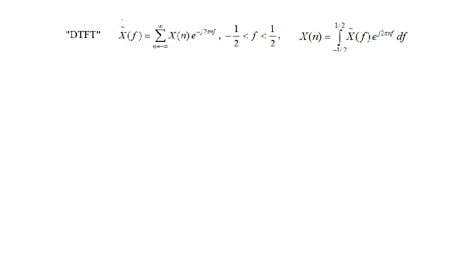

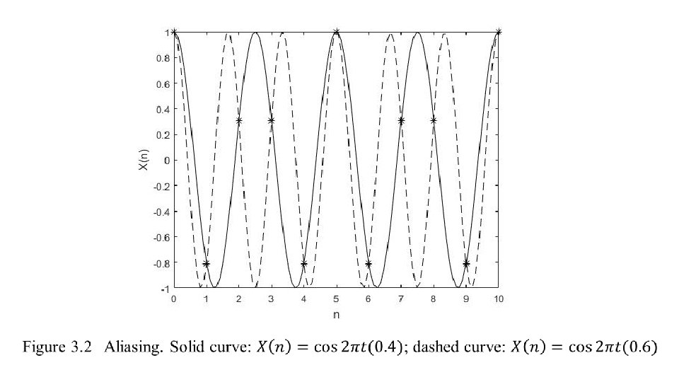
Figure 3. 1 Elements of the Discrete Time Fourier Transform
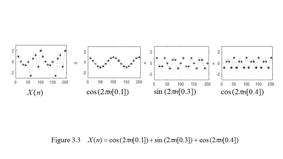
.")
Figure 3. 4 Change of indices in formula (3. 20).

Figure 3. 5 Linear time invariant system responses

Figure 3. 6 Narrow band pass filter
 simulation")
Figure 3. 7 Data from ARMA (2, 1) simulation

Figure 3. 8 Periodogram with frequencies -0. 5 < f < 0. 5 (with true PSD)

Figure 3. 9 Bartlett PSD estimate, -0. 5 < f < 0. 5
 ≡ 4/3, RX(1) ≡ -2/3, RX(2) ≡ 1/3,")
Figure 3. 10 Autocorrelation estimates (RX(0) ≡ 4/3, RX(1) ≡ -2/3, RX(2) ≡ 1/3, RX(3) ≡ -1/6)

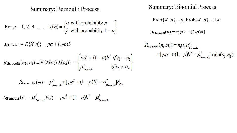
Chapter 4. Models for Random Processes 4. 1 Differential Equations Background 4. 2 Difference Equations 4. 3 ARMA Models 4. 4 The Yule-Walker Equations 4. 5 Construction of ARMA Models 4. 6 Higher-Order ARMA Processes 4. 7 The Random Sine Wave 4. 8 The Bernoulli and Binomial Processes 4. 9 Shot Noise and the Poisson Process 4. 10 Random Walks and the Wiener Process 4. 11 Markov Processes
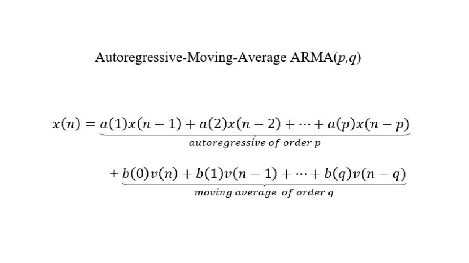

Figure 4. 1. Random Sine Wave
")
Figure 4. 2 Galton machine © UCL Galton Collection (University College London)

Figure 4. 3 m=9 events in an interval T

Figure 4. 4 The Poisson Process

Figure 4. 5 Poisson process and random walk
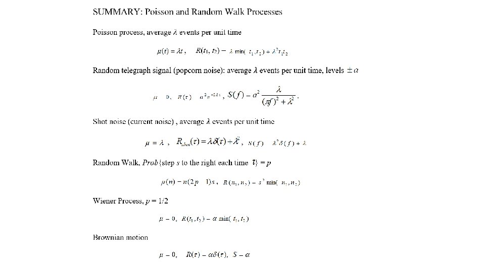

Figure 4. 6 Markov Process

Figure 4. 7 Cyclic Markov Process

Figure 4. 8 Power Spectral Densities

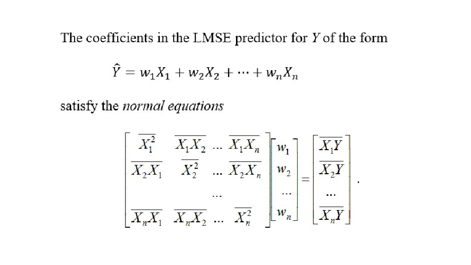
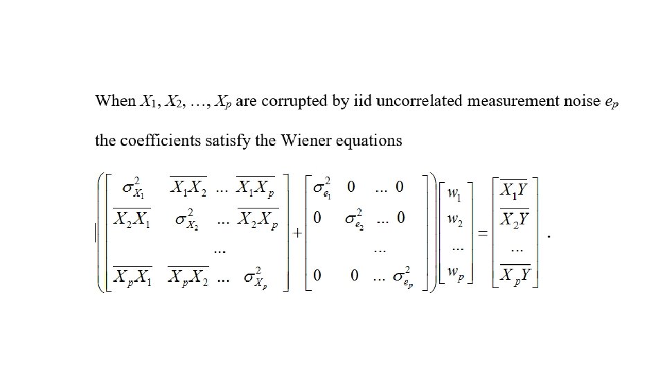
Chapter 5. Least Mean-Square Error Predictors 5. 1 The Optimal Constant Predictor 5. 2 The Optimal Constant-Multiple Predictor 5. 3 Digression: Orthogonality 5. 4 Multivariate LMSE Prediction: The Normal Equations 5. 5 The Bias 5. 6 Best Straight-Line Predictor 5. 7 Prediction for a Random Process 5. 8 Interpolation, Smoothing, Extrapolation, and Back-Prediction 5. 9 The Wiener Filter

Figure 5. 1 Orthogonal Projection

Chapter 6 The Kalman Filter 6. 1 The Basic Kalman Filter 6. 2 Kalman Filter with Transition: Model and Examples 6. 3 The Scalar Kalman Filter with Noiseless Transition 6. 4 The Scalar Kalman Filter with Noisy Transition 6. 5 Iteration of the Scalar Kalman Filter 6. 6 Matrix Formulation for the Kalman Filter
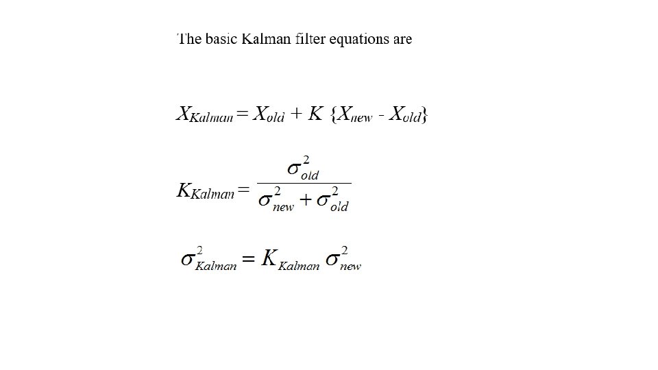
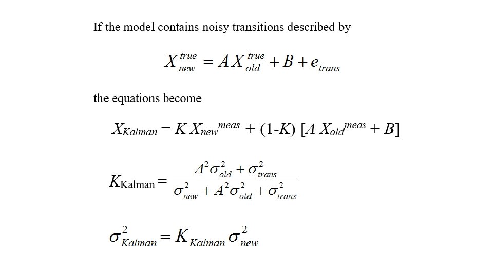

Figure 6. 1 RC circuit

Figure 6. 2 Kalman filter with noisy transition

Figure 6. 3 Consecutive Kalman Filtering

Figure 6. 4 Consecutive Kalman Filtering
![XKalman = K Xnewmeas + (1 -K) [A Xold. Kal + B]](http://slidetodoc.com/presentation_image_h2/ad589c8363faf6fd3840c45efabe467b/image-96.jpg "XKalman = K Xnewmeas + (1 -K) [A Xold. Kal + B]")
XKalman = K Xnewmeas + (1 -K) [A Xold. Kal + B]
![Matrix Formulation XKalman = [AXold. Kal + B] + K[S - D(A Xold. Kal](http://slidetodoc.com/presentation_image_h2/ad589c8363faf6fd3840c45efabe467b/image-97.jpg "Matrix Formulation XKalman = [AXold. Kal + B] + K[S - D(A Xold. Kal")
Matrix Formulation XKalman = [AXold. Kal + B] + K[S - D(A Xold. Kal +B)]
- Slides: 97