Chapter 1 Mathematical Methods with Maple Computer algebra

Chapter 1. Mathematical Methods with Maple • Computer algebra systems in scientific computing (see e. g. J. Gathen, J. Gerhard. Modern Computer Algebra. Cambridge University Press, 1999; M. J. Wester. Computer Algebra Systems: A Practical Guide, John Wiley, 1999) • Maple – an interactive system, allowing one to carry out both numerical and analytical computations. Maple contains 2 D and 3 D graphical means, powerful programming language and an extensive library of mathematical formulae • A convenient working method, when all stages of mathematical, physical or engineering research can be stored in a single document - worksheet • The worksheet automatically becomes a scientific article, report, chapter in a book, etc. Chapter 1. Mathematical Methods with Maple 1

Literature on Maple • A. Heck, Introduction to Maple. Springer, 1996 • M. B. Monagan, K. O. Geddes, K. M. Heal, G. Labahn, S. M. Vorkoetter, J. Mc. Carron. Maple 6. Programming Guide. Waterloo Maple Inc. 2000 • K. M. Heal, M. L. Hansen, K. M. Rickard. Maple 6. Learning Guide. Waterloo Maple Inc. 2000 • D. Redfern. The Maple Handbook. Springer, 1996 • W. Gandler, J. Hrebicek. Solving Problems in Scientific Computing Using Maple and MATLAB. Springer, 1995 • E. Kamerich. A Guide to Maple. Springer, 1999 Chapter 1. Mathematical Methods with Maple 2

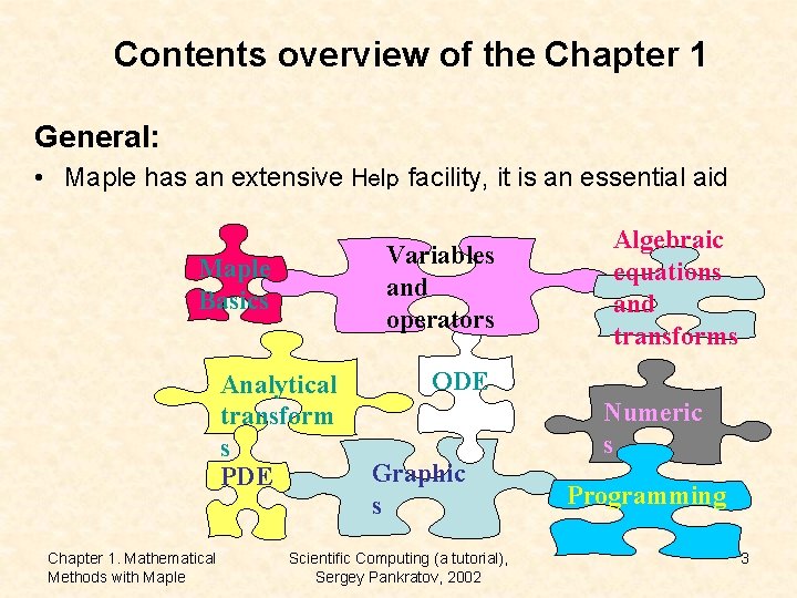
Contents overview of the Chapter 1 General: • Maple has an extensive Help facility, it is an essential aid Variables and operators Maple Basics Analytical transform s PDE Chapter 1. Mathematical Methods with Maple Algebraic equations and transforms ODE Graphic s Scientific Computing (a tutorial), Sergey Pankratov, 2002 Numeric s Programming 3

Document organization in Maple • One should familiarize oneself with Maple GUI • The best way is to learn use and syntax of Maple simultaneously and by examples • A worksheet (*. mws) consists of logical groups called „execution groups“ Each group consists of several parts : - Input Region - Output Region - Text Region (e. g. comments) • The principal objects in Maple: numbers, constants, names - numbers: integer, real, rational, radicals - constants: Pi, I, E, Infinity, gamma, true, false - names: sequences of symbols starting with literal (e. g. new, New, new_old, etc. ) Chapter 1. Mathematical Methods with Maple 4

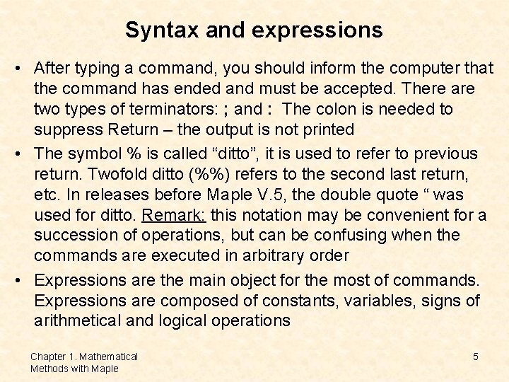
Syntax and expressions • After typing a command, you should inform the computer that the command has ended and must be accepted. There are two types of terminators: ; and : The colon is needed to suppress Return – the output is not printed • The symbol % is called “ditto”, it is used to refer to previous return. Twofold ditto (%%) refers to the second last return, etc. In releases before Maple V. 5, the double quote “ was used for ditto. Remark: this notation may be convenient for a succession of operations, but can be confusing when the commands are executed in arbitrary order • Expressions are the main object for the most of commands. Expressions are composed of constants, variables, signs of arithmetical and logical operations Chapter 1. Mathematical Methods with Maple 5

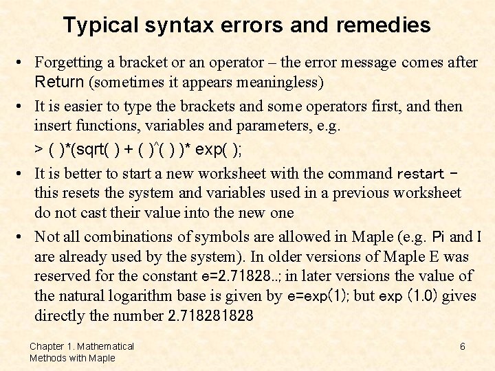
Typical syntax errors and remedies • Forgetting a bracket or an operator – the error message comes after Return (sometimes it appears meaningless) • It is easier to type the brackets and some operators first, and then insert functions, variables and parameters, e. g. > ( )*(sqrt( ) + ( )^( ) )* exp( ); • It is better to start a new worksheet with the command restart – this resets the system and variables used in a previous worksheet do not cast their value into the new one • Not all combinations of symbols are allowed in Maple (e. g. Pi and I are already used by the system). In older versions of Maple E was reserved for the constant e=2. 71828. . ; in later versions the value of the natural logarithm base is given by e=exp(1); but exp (1. 0) gives directly the number 2. 71828 Chapter 1. Mathematical Methods with Maple 6

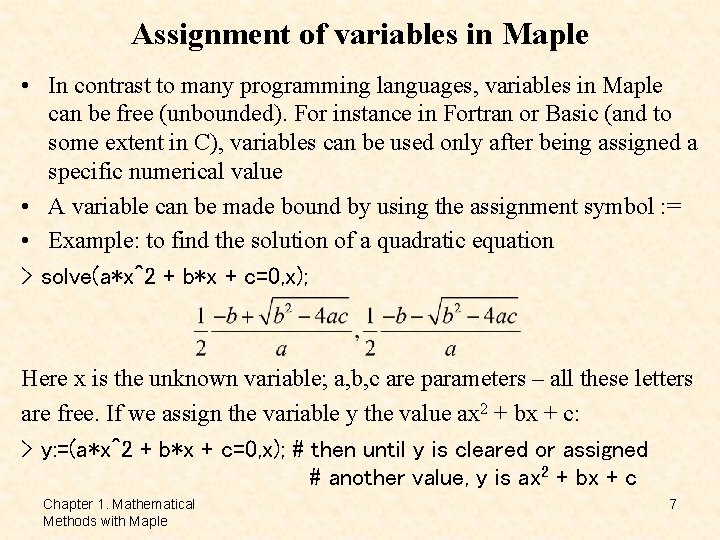
Assignment of variables in Maple • In contrast to many programming languages, variables in Maple can be free (unbounded). For instance in Fortran or Basic (and to some extent in C), variables can be used only after being assigned a specific numerical value • A variable can be made bound by using the assignment symbol : = • Example: to find the solution of a quadratic equation > solve(a*x^2 + b*x + c=0, x); Here x is the unknown variable; a, b, c are parameters – all these letters are free. If we assign the variable y the value ax 2 + bx + c: > y: =(a*x^2 + b*x + c=0, x); # then until y is cleared or assigned # another value, y is ax 2 + bx + c Chapter 1. Mathematical Methods with Maple 7

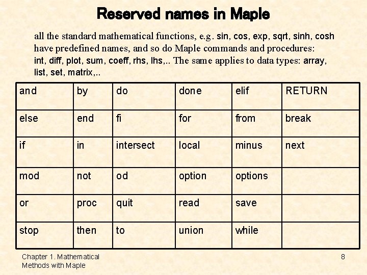
Reserved names in Maple all the standard mathematical functions, e. g. sin, cos, exp, sqrt, sinh, cosh have predefined names, and so do Maple commands and procedures: int, diff, plot, sum, coeff, rhs, lhs, . . The same applies to data types: array, list, set, matrix, . . and by do done elif RETURN else end fi for from break if in intersect local minus next mod not od options or proc quit read save stop then to union while Chapter 1. Mathematical Methods with Maple 8

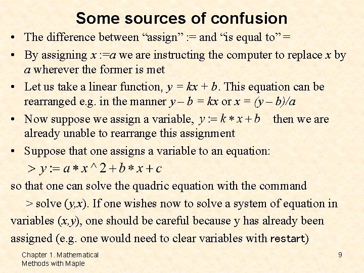
Some sources of confusion • The difference between “assign” : = and “is equal to” = • By assigning x : =a we are instructing the computer to replace x by a wherever the former is met • Let us take a linear function, y = kx + b. This equation can be rearranged e. g. in the manner y – b = kx or x = (y – b)/a • Now suppose we assign a variable, then we are already unable to rearrange this assignment • Suppose that one assigns a variable to an equation: so that one can solve the quadric equation with the command > solve (y, x). If one wishes now to solve a system of equation in variables (x, y), one should be careful because y has already been assigned (e. g. one would need to clear variables with restart) Chapter 1. Mathematical Methods with Maple 9

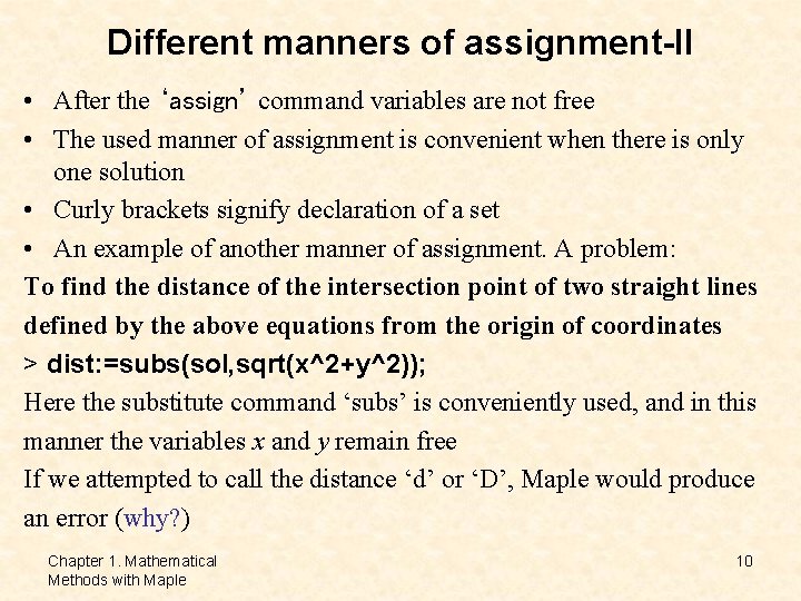
Different manners of assignment-II • After the ‘assign’ command variables are not free • The used manner of assignment is convenient when there is only one solution • Curly brackets signify declaration of a set • An example of another manner of assignment. A problem: To find the distance of the intersection point of two straight lines defined by the above equations from the origin of coordinates > dist: =subs(sol, sqrt(x^2+y^2)); Here the substitute command ‘subs’ is conveniently used, and in this manner the variables x and y remain free If we attempted to call the distance ‘d’ or ‘D’, Maple would produce an error (why? ) Chapter 1. Mathematical Methods with Maple 10

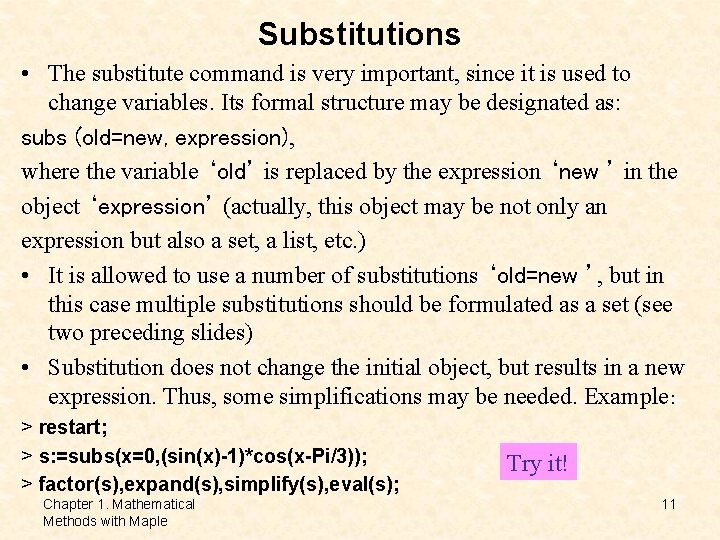
Substitutions • The substitute command is very important, since it is used to change variables. Its formal structure may be designated as: subs (old=new, expression), where the variable ‘old’ is replaced by the expression ‘new ’ in the object ‘expression’ (actually, this object may be not only an expression but also a set, a list, etc. ) • It is allowed to use a number of substitutions ‘old=new ’, but in this case multiple substitutions should be formulated as a set (see two preceding slides) • Substitution does not change the initial object, but results in a new expression. Thus, some simplifications may be needed. Example: > restart; > s: =subs(x=0, (sin(x)-1)*cos(x-Pi/3)); > factor(s), expand(s), simplify(s), eval(s); Chapter 1. Mathematical Methods with Maple Try it! 11

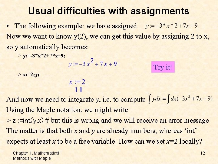
Usual difficulties with assignments • The following example: we have assigned Now we want to know y(2), we can get this value by assigning 2 to x, so y automatically becomes: > y: =-3*x^2+7*x+9; Try it! > x: =2; y; And now we need to integrate y, i. e. to compute Using the Maple notation, we might write > z : =int(y, x) # but this is wrong and we will receive an error message The matter is that both x and y are already numbers, whereas ‘int’ expects at least x to be a free variable. How can we set x=2 locally? Chapter 1. Mathematical Methods with Maple 12

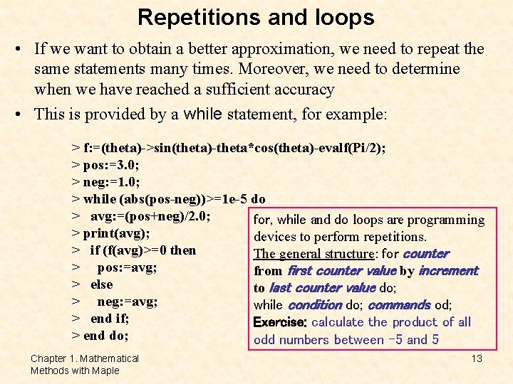
Repetitions and loops • If we want to obtain a better approximation, we need to repeat the same statements many times. Moreover, we need to determine when we have reached a sufficient accuracy • This is provided by a while statement, for example: > f: =(theta)->sin(theta)-theta*cos(theta)-evalf(Pi/2); > pos: =3. 0; > neg: =1. 0; > while (abs(pos-neg))>=1 e-5 do > avg: =(pos+neg)/2. 0; for, while and do loops are programming > print(avg); devices to perform repetitions. > if (f(avg)>=0 then The general structure: for counter > pos: =avg; from first counter value by increment > else to last counter value do; > neg: =avg; while condition do; commands od; > end if; Exercise: calculate the product of all > end do; odd numbers between -5 and 5 Chapter 1. Mathematical Methods with Maple 13

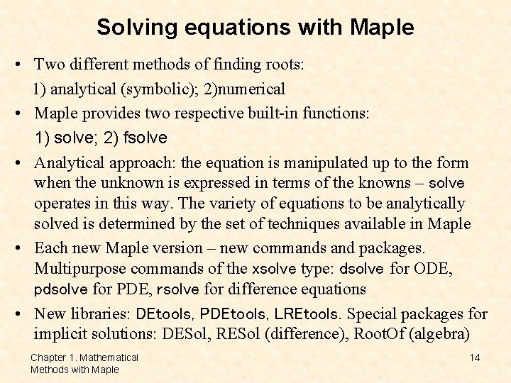
Solving equations with Maple • Two different methods of finding roots: 1) analytical (symbolic); 2)numerical • Maple provides two respective built-in functions: 1) solve; 2) fsolve • Analytical approach: the equation is manipulated up to the form when the unknown is expressed in terms of the knowns – solve operates in this way. The variety of equations to be analytically solved is determined by the set of techniques available in Maple • Each new Maple version – new commands and packages. Multipurpose commands of the xsolve type: dsolve for ODE, pdsolve for PDE, rsolve for difference equations • New libraries: DEtools, PDEtools, LREtools. Special packages for implicit solutions: DESol, RESol (difference), Root. Of (algebra) Chapter 1. Mathematical Methods with Maple 14

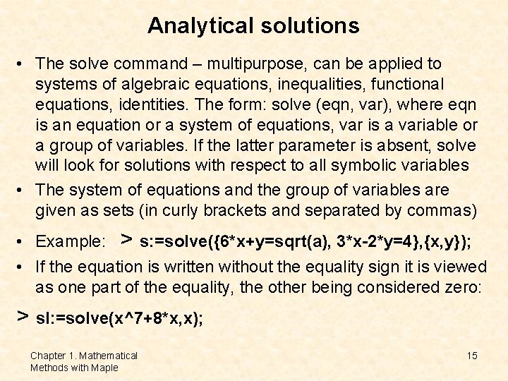
Analytical solutions • The solve command – multipurpose, can be applied to systems of algebraic equations, inequalities, functional equations, identities. The form: solve (eqn, var), where eqn is an equation or a system of equations, var is a variable or a group of variables. If the latter parameter is absent, solve will look for solutions with respect to all symbolic variables • The system of equations and the group of variables are given as sets (in curly brackets and separated by commas) • Example: > s: =solve({6*x+y=sqrt(a), 3*x-2*y=4}, {x, y}); • If the equation is written without the equality sign it is viewed as one part of the equality, the other being considered zero: > sl: =solve(x^7+8*x, x); Chapter 1. Mathematical Methods with Maple 15

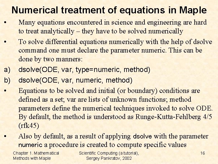
Numerical treatment of equations in Maple • • a) b) • • Many equations encountered in science and engineering are hard to treat analytically – they have to be solved numerically To solve differential equations numerically with the help of dsolve command one must declare the parameter numeric. This can be done by two manners: dsolve(ODE, var, type=numeric, method) dsolve(ODE, var, numeric, method) Equations to be solved and initial (or boundary) conditions are defined as a set; var are lists of unknown functions; method parameters define the numerical techniques invoked to solve ODE. By default, the method is understood as Runge-Kutta-Fehlberg 4/5 (rfk 45) Also by default, as a result of applying dsolve with the parameter numeric a procedure is created to compute specific values Chapter 1. Mathematical Methods with Maple Scientific Computing (a tutorial), Sergey Pankratov, 2002 16

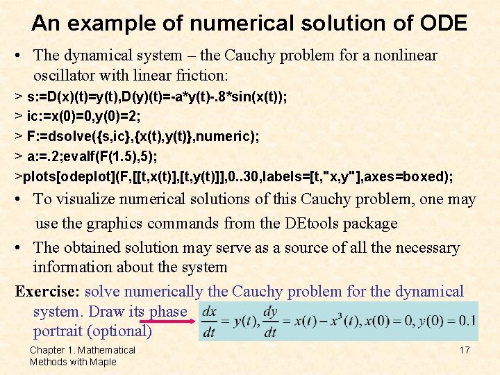
An example of numerical solution of ODE • The dynamical system – the Cauchy problem for a nonlinear oscillator with linear friction: > s: =D(x)(t)=y(t), D(y)(t)=-a*y(t)-. 8*sin(x(t)); > ic: =x(0)=0, y(0)=2; > F: =dsolve({s, ic}, {x(t), y(t)}, numeric); > a: =. 2; evalf(F(1. 5), 5); >plots[odeplot](F, [[t, x(t)], [t, y(t)]], 0. . 30, labels=[t, "x, y"], axes=boxed); • To visualize numerical solutions of this Cauchy problem, one may use the graphics commands from the DEtools package • The obtained solution may serve as a source of all the necessary information about the system Exercise: solve numerically the Cauchy problem for the dynamical system. Draw its phase portrait (optional) Chapter 1. Mathematical Methods with Maple 17

Chapter 2. Mathematical Methods for Modeling • As a rule, real systems and processes are described by nonlinear equations, e. g. differential equations with respect to time and spatial coordinates • Such systems are distributed in space and correspond to an infinite number of degrees of freedom • If the equations modeling the system do not contain spatial derivatives (ODE-based models), such a system is called point-like or having a null-dimension • In the modeling with ODE, each degree of freedom is described by a second-order ODE. Differential equations of the first order correspond to ½ degrees of freedom • The equation du/dt = f(u, t) gives an example of a dynamical system, i. e. the one, whose behavior is uniquely determined by its initial state (deterministic behavior) Chapter 2. Mathematical Methods for Modeling 18

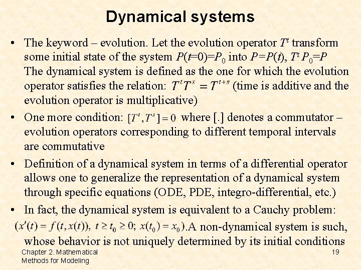
Dynamical systems • The keyword – evolution. Let the evolution operator Tt transform some initial state of the system P(t=0)=P 0 into P=P(t), Tt P 0=P The dynamical system is defined as the one for which the evolution operator satisfies the relation: (time is additive and the evolution operator is multiplicative) • One more condition: where [. ] denotes a commutator – evolution operators corresponding to different temporal intervals are commutative • Definition of a dynamical system in terms of a differential operator allows one to generalize the representation of a dynamical system through specific equations (ODE, PDE, integro-differential, etc. ) • In fact, the dynamical system is equivalent to a Cauchy problem: . A non-dynamical system is such, whose behavior is not uniquely determined by its initial conditions Chapter 2. Mathematical Methods for Modeling 19

The motivation – why bother? • Dynamical systems contain geometric information in the form of a vector field. Interpretation of this geometrical information is the primary means of grasping evolutionary equations. Dynamics is the geometry of behavior • Qualitative analysis of solutions of dynamical systems may provide better understanding than numerical and even analytical calculations • Quantitative investigation of dynamical systems can be readily accompanied by visualization • Asymptotic analysis and long-term numerical exploration: to find the maximal time step still ensuring the closure of the approximate solutions to the exact solution • The exact solution exists (Cauchy-Peano theorem), is unique and continuous on rhs and initial conditions under general assumptions Chapter 2. Mathematical Methods for Modeling 20

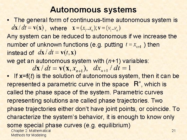
Autonomous systems • The general form of continuous-time autonomous system is , where Any system can be reduced to autonomous if we increase the number of unknown functions (e. g. putting ) then instead of we get an autonomous system with (n+1) variables: • If x=f(t) is the solution of autonomous system, then it can be represented a parametric curve in the space , which is called the phase space of the system. Parametric curves representing solutions are called phase trajectories. Two phase trajectories either don’t have joint points, or coincide. To characterize the system’s behavior, it is enough to know only some special phase curves (e. g. equilibrium) Chapter 2. Mathematical Methods for Modeling 21

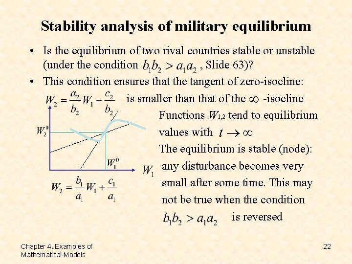
Stability analysis of military equilibrium • Is the equilibrium of two rival countries stable or unstable (under the condition , Slide 63)? • This condition ensures that the tangent of zero-isocline: is smaller than that of the -isocline Functions W 1, 2 tend to equilibrium values with The equilibrium is stable (node): any disturbance becomes very small after some time. This may not be true when the condition is reversed Chapter 4. Examples of Mathematical Models 22

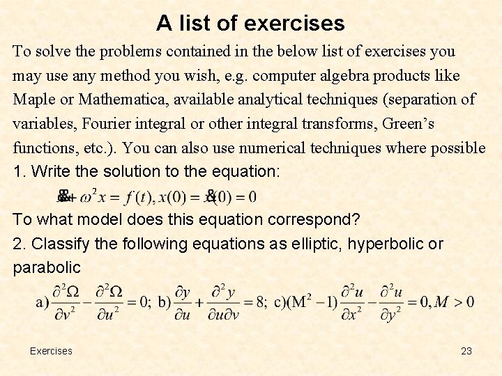
A list of exercises To solve the problems contained in the below list of exercises you may use any method you wish, e. g. computer algebra products like Maple or Mathematica, available analytical techniques (separation of variables, Fourier integral or other integral transforms, Green’s functions, etc. ). You can also use numerical techniques where possible 1. Write the solution to the equation: To what model does this equation correspond? 2. Classify the following equations as elliptic, hyperbolic or parabolic Exercises 23

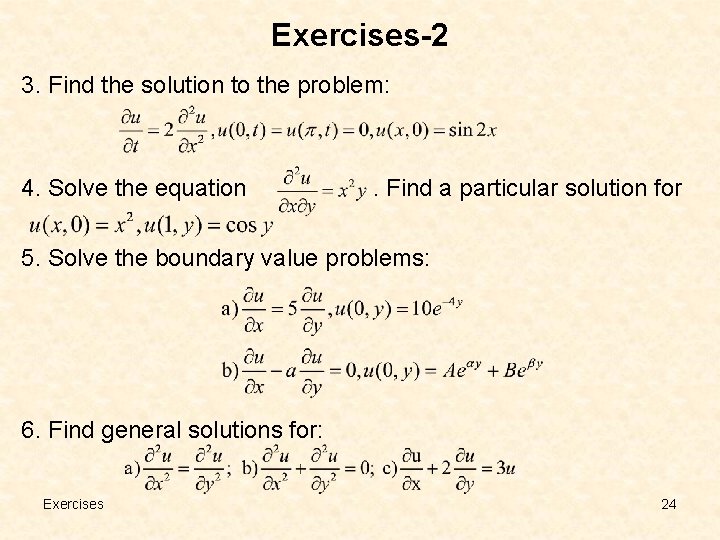
Exercises-2 3. Find the solution to the problem: 4. Solve the equation . Find a particular solution for 5. Solve the boundary value problems: 6. Find general solutions for: Exercises 24

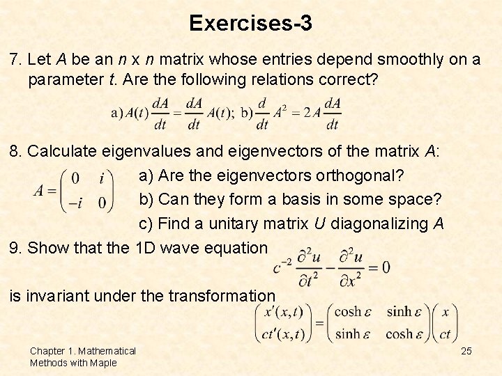
Exercises-3 7. Let A be an n x n matrix whose entries depend smoothly on a parameter t. Are the following relations correct? 8. Calculate eigenvalues and eigenvectors of the matrix A: a) Are the eigenvectors orthogonal? b) Can they form a basis in some space? c) Find a unitary matrix U diagonalizing A 9. Show that the 1 D wave equation is invariant under the transformation Chapter 1. Mathematical Methods with Maple 25

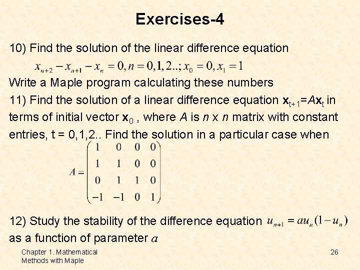
Exercises-4 10) Find the solution of the linear difference equation Write a Maple program calculating these numbers 11) Find the solution of a linear difference equation xt+1=Axt in terms of initial vector x 0 , where A is n x n matrix with constant entries, t = 0, 1, 2. . Find the solution in a particular case when 12) Study the stability of the difference equation as a function of parameter a Chapter 1. Mathematical Methods with Maple 26

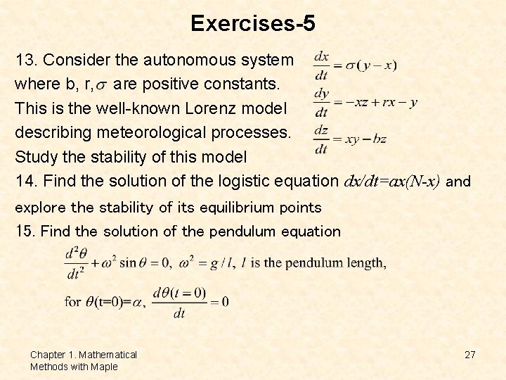
Exercises-5 13. Consider the autonomous system where b, r, are positive constants. This is the well-known Lorenz model describing meteorological processes. Study the stability of this model 14. Find the solution of the logistic equation dx/dt=ax(N-x) and explore the stability of its equilibrium points 15. Find the solution of the pendulum equation Chapter 1. Mathematical Methods with Maple 27