Chapter 1 Introduction Why we are using Computers

Chapter 1 Introduction

Why we are using Computers? • Computers produce fast, accurate and reliable results. • While computers do the boring, repetitive, ordinary tasks, we can spend our efforts and time to work on more interesting and creative tasks. • The use of computers in business and manufacturing decreases the cost of goods and services produced. • It is more difficult and needs more time to find or grow up a skillful labor in industry, while buying an additional computer and installing the required software on is easier and cheaper.

Need for Programming • Computers are just electronic devices that have the power to perform difficult tasks but they do not ‘KNOW’ what to do. • Programmers tell the computers what to do by writing programs

What is Data, Information and Knowledge ? • Data are the raw facts, gathered from the environment which does not have much meaning. • Information is the end product of the processing of data, which has more meaning, and is used in decision making. • Knowledge is the proved and generalized form of information, that is used in strategic planning.

What is a Computer Program? • A computer program is – a set of instructions written in a computer language – executed to perform a specific task. – Also called SOFTWARE • There are tens of programming languages, used nowadays. – C, C++, C#, Pascal, Delphi, Visual Basic, Java, COBOL, FORTRAN, LISP, Prolog …

Properties of Well Designed Programs • Well designed programs must be: – Correct and accurate – Easy to understand – Easy to maintain and update – Efficient – Reliable – Flexible

Steps involved in Programming 1. Requirement Specification: eliminate ambiguities. Clearly understand the problem 2. Analyze the problem : Understand the inputs, outputs and processes used for manipulating the data, formulas and constraints 3. Design: Write the algorithm (flowchart or pseudocode) to represent the solution 4. Testing and verification : Check the algorithm. 5. Implement the algorithm : Write a program 6. Testing and Verification: Check the program 7. Documentation

What is an Algorithm? • It is a sequence of executed, unambiguous instructions for solving a problem (i. e. obtained the required output for any instance of input in a finite amount of time)

Algorithm An algorithm is a method of solving problem (on a computer) • The range of inputs for which an algorithm works must be specified carefully. • The same algorithm can be represented in several ways. • For same problem, several algorithms may exists. • Algorithms solving same problem can be based on different ideas and have dramatically different speeds. 9

Examples: : Greatest common divisor - gcd Algorithm 1 • Problem: For two nonnegative, not-both-zero integers m and n, find largest integer that divides both of them evenly, i. e. , with a remainder of a zero. • Solution: Euclid’s algorithm Apply repeatedly gcd ( m, n ) = gcd ( n, m mod n ) gcd(60, 24) = 12, gcd(60, 0) = 60, gcd(0, 0) = ? • Example: gcd(60, 24) = gcd(24, 12) = gcd(12, 0) = 12 Euclid’s algorithm for computing gcd( m, n). 1. If n=0, return the value of m as answer and stop; otherwise proceed to 2. 2. Divide m by n and assign value of the reminder to r. 3. Assign the value of n to m and the value of r to n. Go to 1. 10

Consecutive integer checking Another algorithm to compute gcd ( m, n) 1. Assign the value of min{m, n} to t 2. Divide m by t. If the reminder is 0 go to 3; otherwise go to 4. 3. Divide n by t. If the reminder is 0, return the t as answer and stop; otherwise go to 4. 4. Decrease value of t by 1. Go to 2. 11

Basic Issues Related to Algorithms • • How to design algorithms How to express algorithms Proving correctness Efficiency – Theoretical analysis – Empirical analysis Algorithm design strategies • • Brute force Divide and conquer Decrease and conquer Transform and conquer • Greedy approach • Dynamic programming • Space and time tradeoffs 12

Analysis of Algorithms • How good is the algorithm? – Correctness – Time efficiency – Space efficiency • Algorithms Must be 1. Finiteness bterminates after a finite number of steps 2. Definiteness bunderstanding specified 3. Input bvalid inputs are clearly specified 4. Output bcan be proved to produce the correct output given a valid input 5. Effectiveness bsteps are sufficiently simple and basic 13

Correctness • Termination • Well-founded sets: find a quantity that is never negative and that always decreases as the algorithm is executed • Partial Correctness • For recursive algorithms: induction • For iterative algorithms: loop invariants Complexity • Space complexity • Time complexity - For iterative algorithms: sums - For recursive algorithms: recurrence relations 14

To design algorithm we must: • Understanding the problem There are some types of problems that appears in computer science often. Perhaps there exists algorithms to solve problem you have if you look closely enough. Input of particular algorithm defines instance of the problem. It is important to specify carefully the range of possible inputs to algorithm. • Sure that you have capabilities of computational device Traditionally, algorithms are sequential. It is more natural for humans to think that way. The parallel algorithms are possible in case the computer allows us to do so. Amount of memory algorithm uses may or may not be issue. Speed of computer is relative. • choosing between exact and approximation problem solving Why to choose approximate algorithm? - exact one may take too much time (traveling salesman problem) - problem can not be solved exactly - approximation can be part of more complex exact algorithm 15

Steps for designing and analyzing Algo. • Understanding the problem -read description carefully - ask questions - do few examples -think about special cases 16

Steps for designing and analyzing Algo. • Exact VS. Approximate solution -why we use approximate? -some cases has no exact solution -exact may be very slow -it may be part of complex algorithm that solve the problem exactly 17

Steps for designing and analyzing Algo. • Design algorithm – some techniques may inapplicable – some techniques can be combined with another to form the required technique – sometimes you should decide the data structure used for algo – Algo+Data structure = comp. Program – You should represent the algo by • • - pseudo code -natural language -comp. program -flow chart 18

Steps for designing and analyzing Algo. • Correctness – insure that the algo leads the required results for specified inputs – prove if the algo is stop or not – Normally used Math Induction to prove correctness – use one instance of input that prove the error 19

Steps for designing and analyzing Algo. • Analyzing algo. – *time efficiency – *space(memory) efficiency – simplicity: – simpler is easier to understand – sometimes simpler is more efficient than complex but not always true – generality of the problem 20

Steps for designing and analyzing Algo. • Coding – program should be valid (testing) – The code needs to be optimized – Optimality: Minimum amount of work an algo will need to solve the problem – Rule: a good algo is a result of repeated efforts & rework – if your algo is perfect , you should try to see whether it can be improved 21

Important problem types 1) sorting problem • properties of sorting algo – stable sorting algo X item in pos i and j : i<j after sorting X is in pos i' and j' : i'<j' it is called stable sort • b. In-Place sort • - doesn't need extra memory locations except few memory units (constant amount om memory) 22

2) searching 3) string processing – string matching – compilation 4) Graph problems 5) combinatorial problems 6) Geometric problems: Closest pair , convex hull polygon 7) numerical problems 23

• Deciding the data structures Some algorithms do not have information of representation of their input. Others require some nontrivial organization of input data. Some algorithm design techniques are based on structuring and restructuring data (heap sort for example). We will see how different algorithms uses different data structures. • Algorithm designing techniques • • - Natural language Pseudocode the mixture of programming like constructs and natural language Used flowcarts • Proving an algorithm’s correctness Once you create algorithm you must prove that it is correct. Mathematical induction is often used. We usually want to show that error produced is lowerthen predefined limit. 24

How fast will your program run? • The running time of your program will depend upon: – The algorithm – The input – Your implementation of the algorithm in a programming language – The compiler you use – The OS on your computer – Your computer hardware – Maybe other things: temperature outside; other programs on your computer; … • Our Motivation: analyze the running time of an algorithm as a function of only simple parameters of the input.

Different time functions

Linear Data Structures • Arrays – A sequence of n items of the same data type that are stored contiguously in computer memory and made accessible by specifying a value of the array’s index. • Linked List – A sequence of zero or more nodes each containing two kinds of information: some data and one or more links called pointers to other nodes of the linked list. – Singly linked list (next pointer) – Doubly linked list (next + previous pointers) n Arrays n n n fixed length (need preliminary reservation of memory) contiguous memory locations direct access Insert/delete Linked Lists n n dynamic length arbitrary memory locations access by following links Insert/delete 27

Stacks and Queues • Stacks – A stack of plates • insertion/deletion can be done only at the top. • LIFO – Two operations (push and pop) • Queues – A queue of customers waiting for services • Insertion/enqueue from the rear and deletion/dequeue from the front. • FIFO – Two operations (enqueue and dequeue) 28

Priority Queue and Heap n Priority queues (implemented using heaps) A data structure for maintaining a set of elements, each associated with a key/priority, with the following operations n n n Finding the element with the highest priority n Deleting the element with the highest priority n Inserting a new element Scheduling jobs on computer. 9 6 5 2 8 3 9 6 8 5 229 3

Graphs • Formal definition – A graph G = <V, E> is defined by a pair of two sets: a finite set V of items called vertices and a set E of vertex pairs called edges. • Undirected and directed graphs (digraphs). • What’s the maximum number of edges in an undirected graph with |V| vertices? • Complete: A graph with every pair of its vertices connected by an edge is called complete, K|V| • dense graph has few possible edges missing • sparse graph: # of edges are close to the minimal # of edges 1 2 3 4 30

Graph Representation • Adjacency matrix – n x n boolean matrix if |V| is n. – The element on the ith row and jth column is 1 if there’s an edge from ith vertex to the jth vertex; otherwise 0. – The adjacency matrix of an undirected graph is symmetric. • Adjacency linked lists – A collection of linked lists, one for each vertex, that contain all the vertices adjacent to the list’s vertex. * List is better for Sparse graph • matrix is better for dense graph Weighted Graph: it 0 is 1 a 1 graph with numbers 1 2 3 assign 4 to 4 0 0 1 or cost it's edge and it calls 0 weight 4 0001 0000 31

Path & Cycles • a path from vertex u to v of G is a sequence of adjacent vertices starts from u and end with v • path (a, d): (a, b), (b, d) • length of path = # of edges or # of vertices -1 • simple path : all vertices are distinct • Connected graph: if there is a path for every pair of its vertices u, v is called connected • if one pair has no path it is disconnected graph • Cycle: is a path of a positive length that starts & ends at the same vertex and doesn't traverse the same edge twice or more 32 • if no such a path it is called Acyclic graph

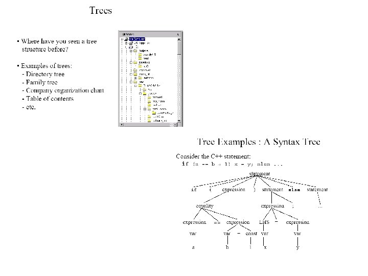
Trees • Trees – A tree (or free tree) is a connected acyclic graph. – Forests: a graph that has no cycles but is not necessarily connected. • Properties of trees – For every two vertices in a tree there always exists exactly one simple path from one of these vertices to the other. Why? • Rooted trees: The above property makes it possible to select an arbitrary vertex in a free tree and consider it as the root of the so called rooted tree. rooted • Levels in a rooted tree. n |E| = |V| - 1 1 3 2 4 5 3 4 1 2 5 33

Data Structures Linear data structures • Array is a sequence of n items of the same data type that are stored contiguously in memory and are accessible by index of array. • String, the array containing characters of alphabet. • Linked list is sequence of zero or more elements – nodes containing some data and one or more pointers to other nodes of the list. • Singly linked list – each node except last one has one pointer to next element • Header is the first element of the list. • Doubly linked list – each node except first and last has two pointers to next and previous element 34

• Stack – it is a list where insert (push) and delete (pop) happens only on one end (LIFO – last in first out). This end is called top • Queue – is a list where elements are inserted on one and deleted on other end (FIFO – first in first out). Front – elements are deleted here – dequeue Rear – elements are inserted here – enqueue • Priority queue – dequeue returns the largest element in queue. Nonlinear data structures Graphs : the most important type. Trees Sets, dictionaries 35