CHAPTER 1 Graphs Functions and Models 1 1

CHAPTER 1: Graphs, Functions, and Models 1. 1 1. 2 1. 3 1. 4 1. 5 1. 6 Introduction to Graphing Functions and Graphs Linear Functions, Slope, and Applications Equations of Lines and Modeling Linear Equations, Functions, Zeros and Applications Solving Linear Inequalities Copyright © 2009 Pearson Education, Inc.

1. 3 Linear Functions, Slope, and Applications · · · Determine the slope of a line given two points on the line. Solve applied problems involving slope. Find the slope and the y-intercept of a line given the equation y = mx + b, or f (x) = mx + b. Graph a linear equation using the slope and the yintercept. Solve applied problems involving linear functions. Copyright © 2009 Pearson Education, Inc.

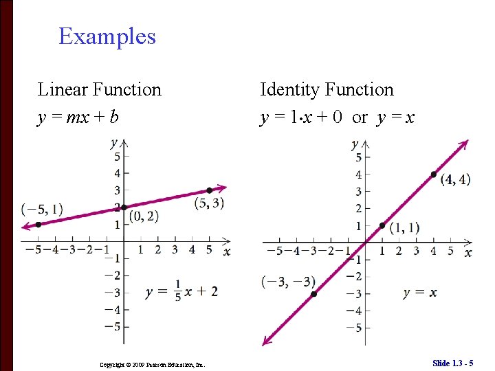
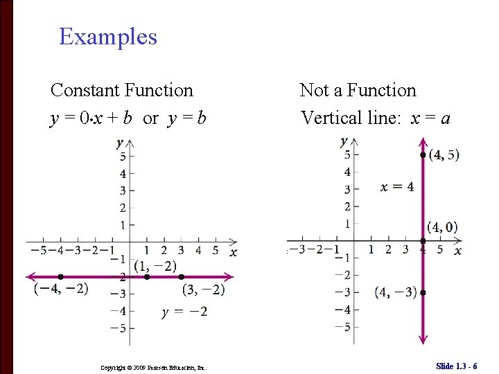
Linear Functions A function f is a linear function if it can be written as f (x) = mx + b, where m and b are constants. If m = 0, the function is a constant function f (x) = b. If m = 1 and b = 0, the function is the identity function f (x) = x. Copyright © 2009 Pearson Education, Inc. Slide 1. 3 - 4

Examples Linear Function y = mx + b Copyright © 2009 Pearson Education, Inc. Identity Function y = 1 • x + 0 or y = x Slide 1. 3 - 5

Examples Constant Function y = 0 • x + b or y = b Copyright © 2009 Pearson Education, Inc. Not a Function Vertical line: x = a Slide 1. 3 - 6

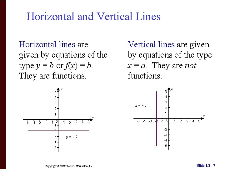
Horizontal and Vertical Lines Horizontal lines are given by equations of the type y = b or f(x) = b. They are functions. Vertical lines are given by equations of the type x = a. They are not functions. x= 2 y= 2 Copyright © 2009 Pearson Education, Inc. Slide 1. 3 - 7

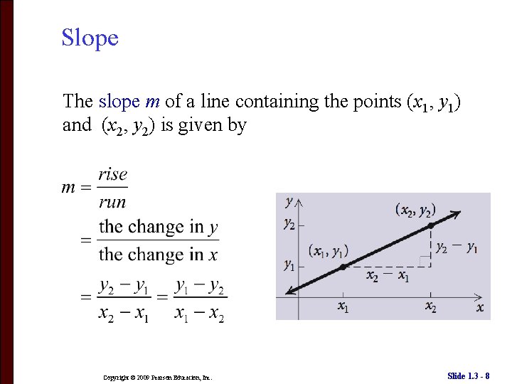
Slope The slope m of a line containing the points (x 1, y 1) and (x 2, y 2) is given by Copyright © 2009 Pearson Education, Inc. Slide 1. 3 - 8

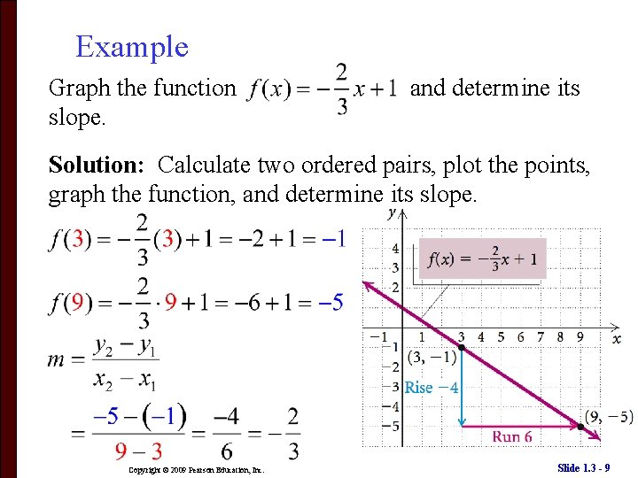
Example Graph the function slope. and determine its Solution: Calculate two ordered pairs, plot the points, graph the function, and determine its slope. Copyright © 2009 Pearson Education, Inc. Slide 1. 3 - 9

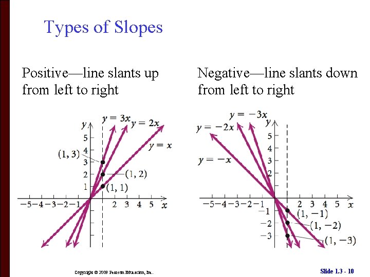
Types of Slopes Positive—line slants up from left to right Copyright © 2009 Pearson Education, Inc. Negative—line slants down from left to right Slide 1. 3 - 10

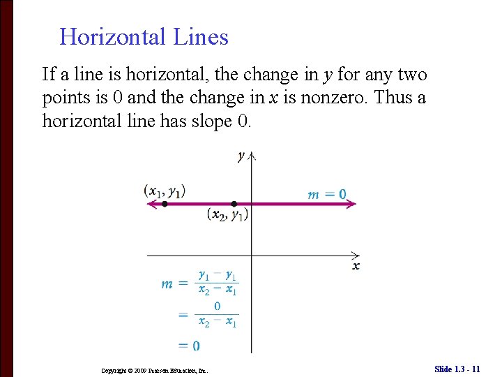
Horizontal Lines If a line is horizontal, the change in y for any two points is 0 and the change in x is nonzero. Thus a horizontal line has slope 0. Copyright © 2009 Pearson Education, Inc. Slide 1. 3 - 11

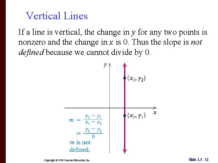
Vertical Lines If a line is vertical, the change in y for any two points is nonzero and the change in x is 0. Thus the slope is not defined because we cannot divide by 0. Copyright © 2009 Pearson Education, Inc. Slide 1. 3 - 12

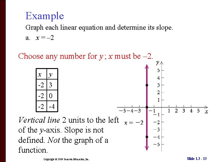
Example Graph each linear equation and determine its slope. a. x = – 2 Choose any number for y ; x must be – 2. x -2 -2 -2 y 3 0 -4 Vertical line 2 units to the left of the y-axis. Slope is not defined. Not the graph of a function. Copyright © 2009 Pearson Education, Inc. Slide 1. 3 - 13

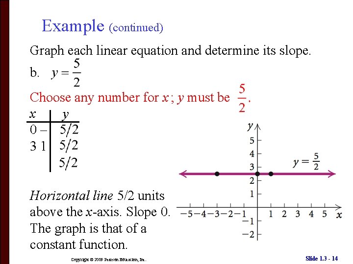
Example (continued) Graph each linear equation and determine its slope. b. Choose any number for x ; y must be x y 0– 31 Horizontal line 5/2 units above the x-axis. Slope 0. The graph is that of a constant function. Copyright © 2009 Pearson Education, Inc. Slide 1. 3 - 14

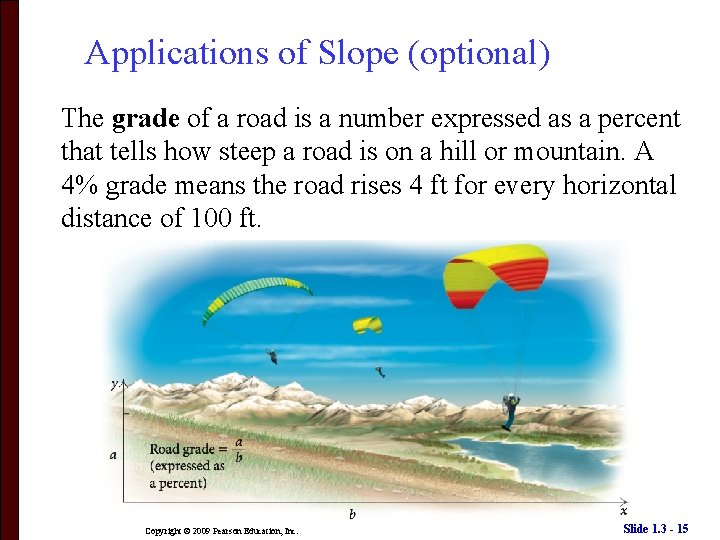
Applications of Slope (optional) The grade of a road is a number expressed as a percent that tells how steep a road is on a hill or mountain. A 4% grade means the road rises 4 ft for every horizontal distance of 100 ft. Copyright © 2009 Pearson Education, Inc. Slide 1. 3 - 15

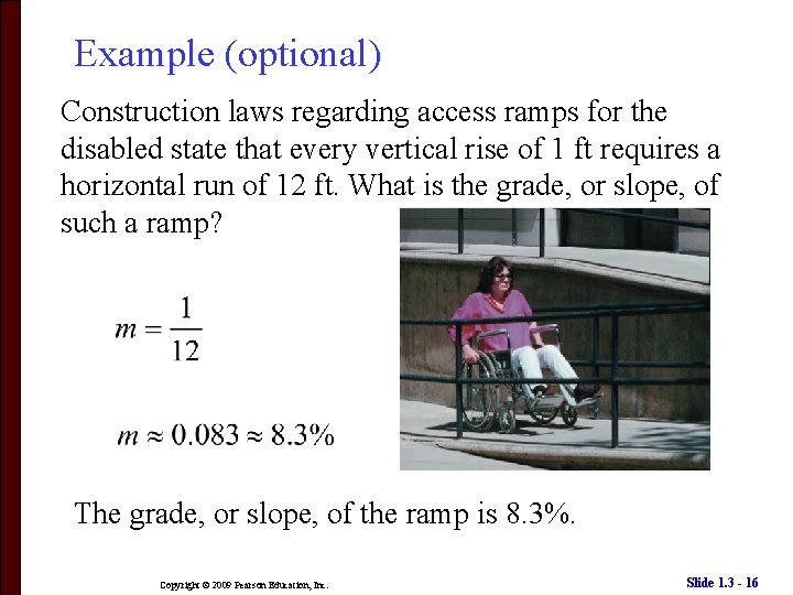
Example (optional) Construction laws regarding access ramps for the disabled state that every vertical rise of 1 ft requires a horizontal run of 12 ft. What is the grade, or slope, of such a ramp? The grade, or slope, of the ramp is 8. 3%. Copyright © 2009 Pearson Education, Inc. Slide 1. 3 - 16

Average Rate of Change (optional) Slope can also be considered as an average rate of change. To find the average rate of change between any two data points on a graph, we determine the slope of the line that passes through the two points. Copyright © 2009 Pearson Education, Inc. Slide 1. 3 - 17

Example (optional) The percent of travel bookings online has increased from 6% in 1999 to 55% in 2007. The graph below illustrates this trend. Find the average rate of change in the percent of travel bookings made online from 1999 to 2007. Copyright © 2009 Pearson Education, Inc. Slide 1. 3 - 18

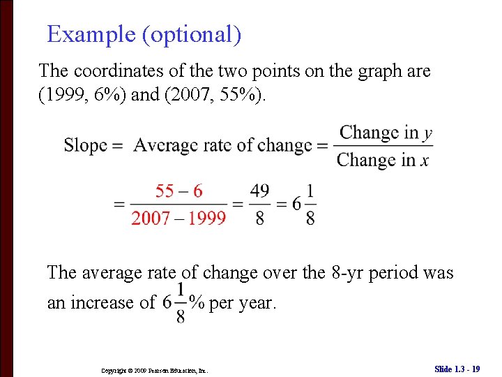
Example (optional) The coordinates of the two points on the graph are (1999, 6%) and (2007, 55%). The average rate of change over the 8 -yr period was an increase of Copyright © 2009 Pearson Education, Inc. per year. Slide 1. 3 - 19

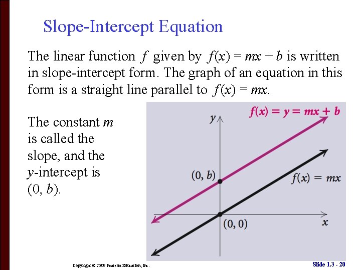
Slope-Intercept Equation The linear function f given by f (x) = mx + b is written in slope-intercept form. The graph of an equation in this form is a straight line parallel to f (x) = mx. The constant m is called the slope, and the y-intercept is (0, b). Copyright © 2009 Pearson Education, Inc. Slide 1. 3 - 20

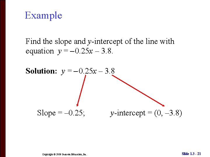
Example Find the slope and y-intercept of the line with equation y = – 0. 25 x – 3. 8. Solution: y = – 0. 25 x – 3. 8 Slope = – 0. 25; Copyright © 2009 Pearson Education, Inc. y-intercept = (0, – 3. 8) Slide 1. 3 - 21

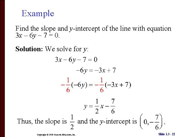
Example Find the slope and y-intercept of the line with equation 3 x – 6 y 7 = 0. Solution: We solve for y: Thus, the slope is Copyright © 2009 Pearson Education, Inc. and the y-intercept is Slide 1. 3 - 22

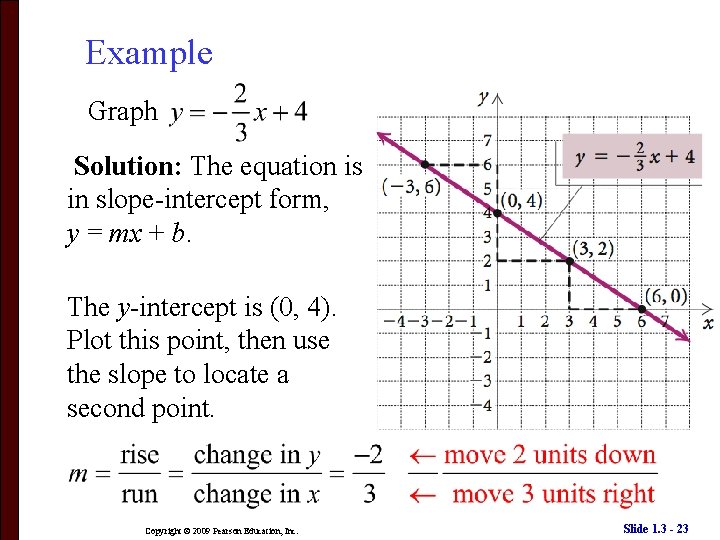
Example Graph Solution: The equation is in slope-intercept form, y = mx + b. The y-intercept is (0, 4). Plot this point, then use the slope to locate a second point. Copyright © 2009 Pearson Education, Inc. Slide 1. 3 - 23

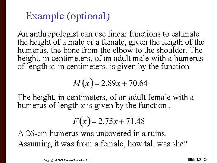
Example (optional) An anthropologist can use linear functions to estimate the height of a male or a female, given the length of the humerus, the bone from the elbow to the shoulder. The height, in centimeters, of an adult male with a humerus of length x, in centimeters, is given by the function The height, in centimeters, of an adult female with a humerus of length x is given by the function. A 26 -cm humerus was uncovered in a ruins. Assuming it was from a female, how tall was she? Copyright © 2009 Pearson Education, Inc. Slide 1. 3 - 24

Example (optional) Solution: We substitute into the function: Thus, the female was 142. 98 cm tall. Copyright © 2009 Pearson Education, Inc. Slide 1. 3 - 25