Chapter 1 Functions and Their Graphs Larson Precalculus

Chapter 1 Functions and Their Graphs Larson, Precalculus, 10 th Edition. © 2018 Cengage. All Rights Reserved. May not be scanned, copied or duplicated, or posted to a publicly accessible website, in whole or in part.

1. 5 Analyzing Graphs of Functions Larson, Precalculus, 10 th Edition. © 2018 Cengage. All Rights Reserved. May not be scanned, copied or duplicated, or posted to a publicly accessible website, in whole or in part.

Objectives • Use the Vertical Line Test for functions. • Find the zeros of functions. • Determine intervals on which functions are increasing or decreasing and determine relative maximum and relative minimum values of functions. • Determine the average rate of change of a function. • Identify even and odd functions. Larson, Precalculus, 10 th Edition. © 2018 Cengage. All Rights Reserved. May not be scanned, copied or duplicated, or posted to a publicly accessible website, in whole or in part.

The Graph of a Function Larson, Precalculus, 10 th Edition. © 2018 Cengage. All Rights Reserved. May not be scanned, copied or duplicated, or posted to a publicly accessible website, in whole or in part.

The Graph of a Function (1 of 5) We have studied functions from an algebraic point of view. In this section, you will study functions from a graphical perspective. The graph of a function f is the collection of ordered pairs (x, f(x)) such that x is in the domain of f. Larson, Precalculus, 10 th Edition. © 2018 Cengage. All Rights Reserved. May not be scanned, copied or duplicated, or posted to a publicly accessible website, in whole or in part.

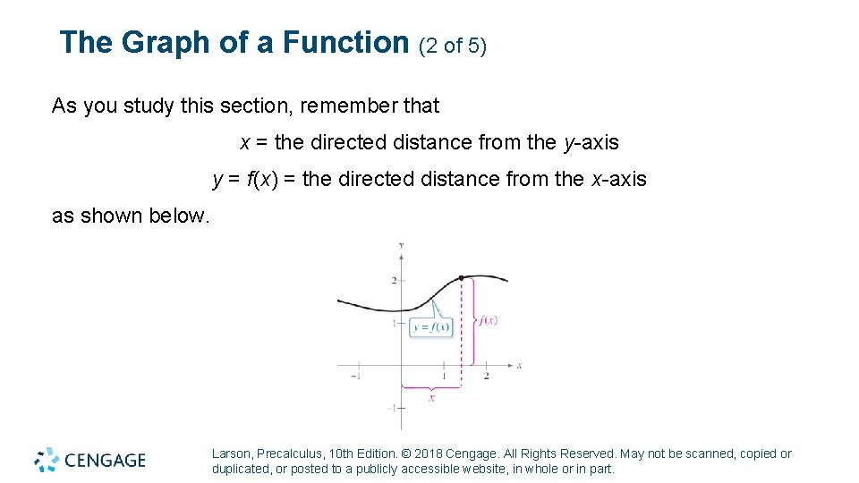
The Graph of a Function (2 of 5) As you study this section, remember that x = the directed distance from the y-axis y = f(x) = the directed distance from the x-axis as shown below. Larson, Precalculus, 10 th Edition. © 2018 Cengage. All Rights Reserved. May not be scanned, copied or duplicated, or posted to a publicly accessible website, in whole or in part.

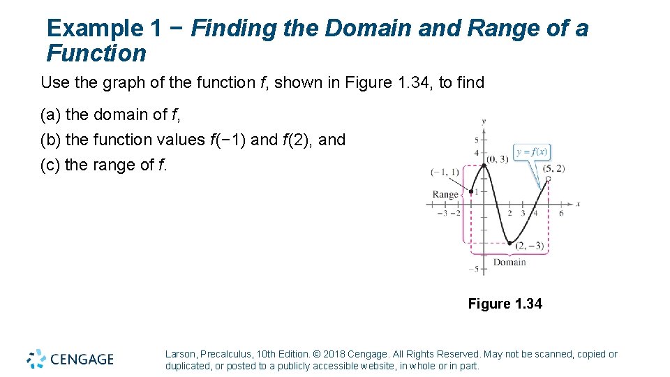
Example 1 − Finding the Domain and Range of a Function Use the graph of the function f, shown in Figure 1. 34, to find (a) the domain of f, (b) the function values f (− 1) and f (2), and (c) the range of f. Figure 1. 34 Larson, Precalculus, 10 th Edition. © 2018 Cengage. All Rights Reserved. May not be scanned, copied or duplicated, or posted to a publicly accessible website, in whole or in part.

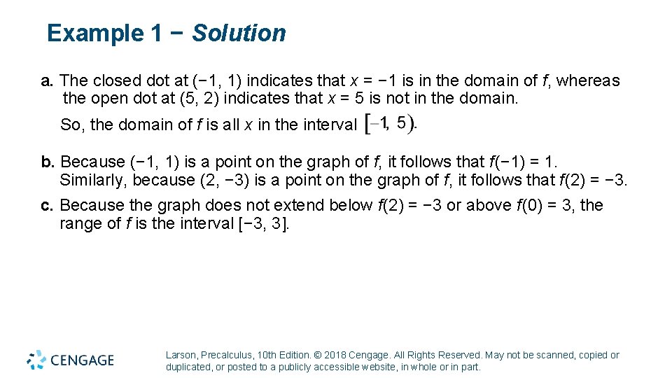
Example 1 − Solution a. The closed dot at (− 1, 1) indicates that x = − 1 is in the domain of f, whereas the open dot at (5, 2) indicates that x = 5 is not in the domain. So, the domain of f is all x in the interval b. Because (− 1, 1) is a point on the graph of f, it follows that f (− 1) = 1. Similarly, because (2, − 3) is a point on the graph of f, it follows that f (2) = − 3. c. Because the graph does not extend below f (2) = − 3 or above f (0) = 3, the range of f is the interval [− 3, 3]. Larson, Precalculus, 10 th Edition. © 2018 Cengage. All Rights Reserved. May not be scanned, copied or duplicated, or posted to a publicly accessible website, in whole or in part.

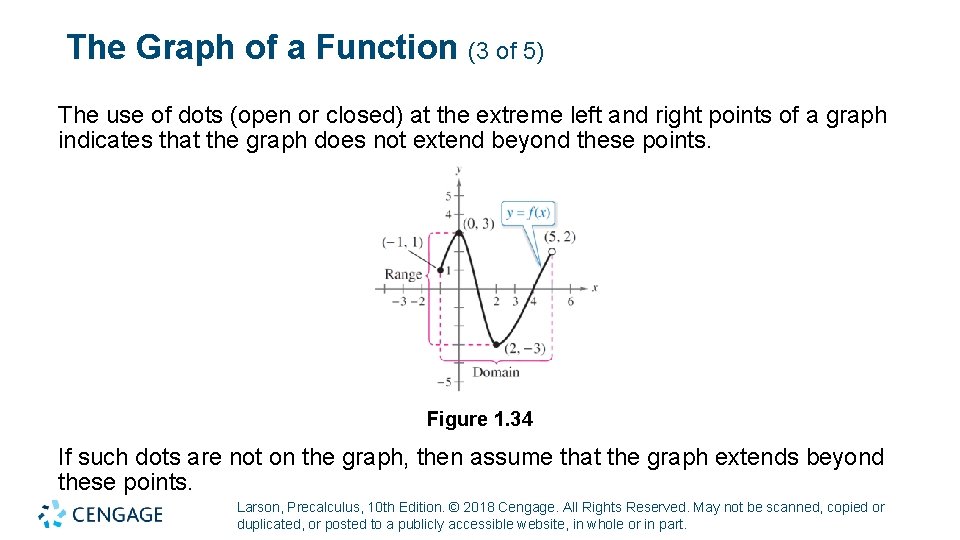
The Graph of a Function (3 of 5) The use of dots (open or closed) at the extreme left and right points of a graph indicates that the graph does not extend beyond these points. Figure 1. 34 If such dots are not on the graph, then assume that the graph extends beyond these points. Larson, Precalculus, 10 th Edition. © 2018 Cengage. All Rights Reserved. May not be scanned, copied or duplicated, or posted to a publicly accessible website, in whole or in part.

The Graph of a Function (4 of 5) By the definition of a function, at most one y-value corresponds to a given xvalue. This means that the graph of a function cannot have two or more different points with the same x-coordinate, and no two points on the graph of a function can be vertically above or below each other. It follows, then, that a vertical line can intersect the graph of a function at most once. Larson, Precalculus, 10 th Edition. © 2018 Cengage. All Rights Reserved. May not be scanned, copied or duplicated, or posted to a publicly accessible website, in whole or in part.

The Graph of a Function (5 of 5) This observation provides a convenient visual test called the Vertical Line Test for functions. Vertical Line Test for Functions A set of points in a coordinate plane is the graph of y as a function of x if and only if no vertical line intersects the graph at more than one point. Larson, Precalculus, 10 th Edition. © 2018 Cengage. All Rights Reserved. May not be scanned, copied or duplicated, or posted to a publicly accessible website, in whole or in part.

Zeros of a Function Larson, Precalculus, 10 th Edition. © 2018 Cengage. All Rights Reserved. May not be scanned, copied or duplicated, or posted to a publicly accessible website, in whole or in part.

Zeros of a Function If the graph of a function of x has an x-intercept at (a, 0), then a is a zero of the function. Zeros of a Function The zeros of a function f of x are the x-values for which f(x) = 0. Larson, Precalculus, 10 th Edition. © 2018 Cengage. All Rights Reserved. May not be scanned, copied or duplicated, or posted to a publicly accessible website, in whole or in part.

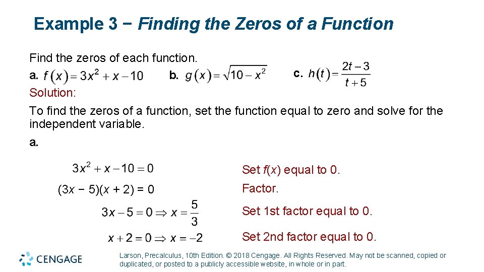
Example 3 − Finding the Zeros of a Function Find the zeros of each function. c. a. b. Solution: To find the zeros of a function, set the function equal to zero and solve for the independent variable. a. Set f(x) equal to 0. (3 x − 5)(x + 2) = 0 Factor. Set 1 st factor equal to 0. Set 2 nd factor equal to 0. Larson, Precalculus, 10 th Edition. © 2018 Cengage. All Rights Reserved. May not be scanned, copied or duplicated, or posted to a publicly accessible website, in whole or in part.

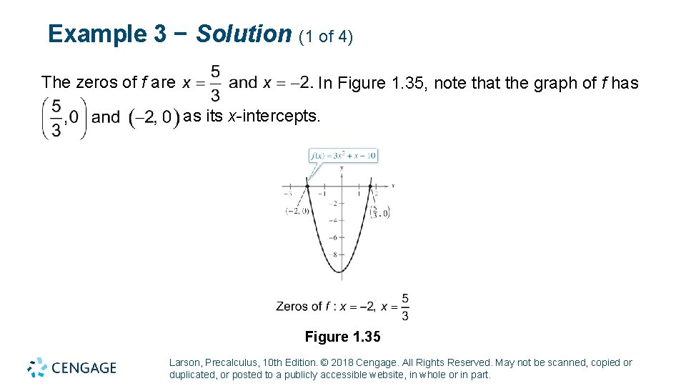
Example 3 − Solution (1 of 4) The zeros of f are In Figure 1. 35, note that the graph of f has as its x-intercepts. Figure 1. 35 Larson, Precalculus, 10 th Edition. © 2018 Cengage. All Rights Reserved. May not be scanned, copied or duplicated, or posted to a publicly accessible website, in whole or in part.

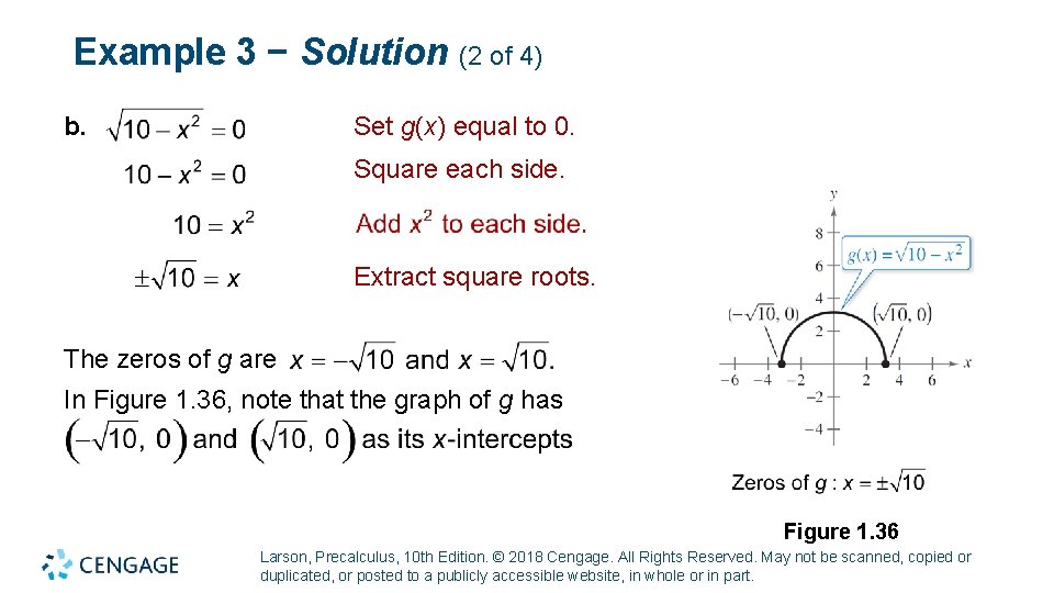
Example 3 − Solution (2 of 4) b. Set g(x) equal to 0. Square each side. Extract square roots. The zeros of g are In Figure 1. 36, note that the graph of g has Figure 1. 36 Larson, Precalculus, 10 th Edition. © 2018 Cengage. All Rights Reserved. May not be scanned, copied or duplicated, or posted to a publicly accessible website, in whole or in part.

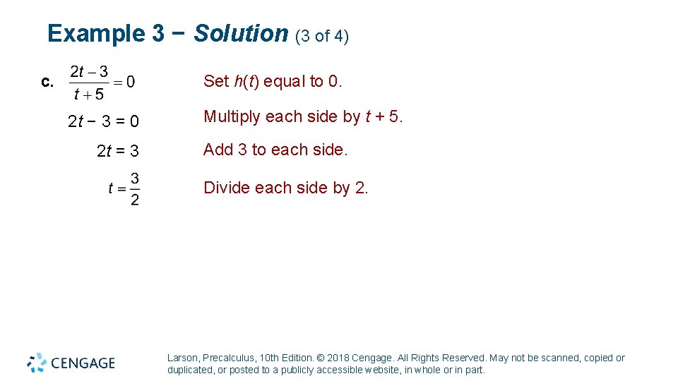
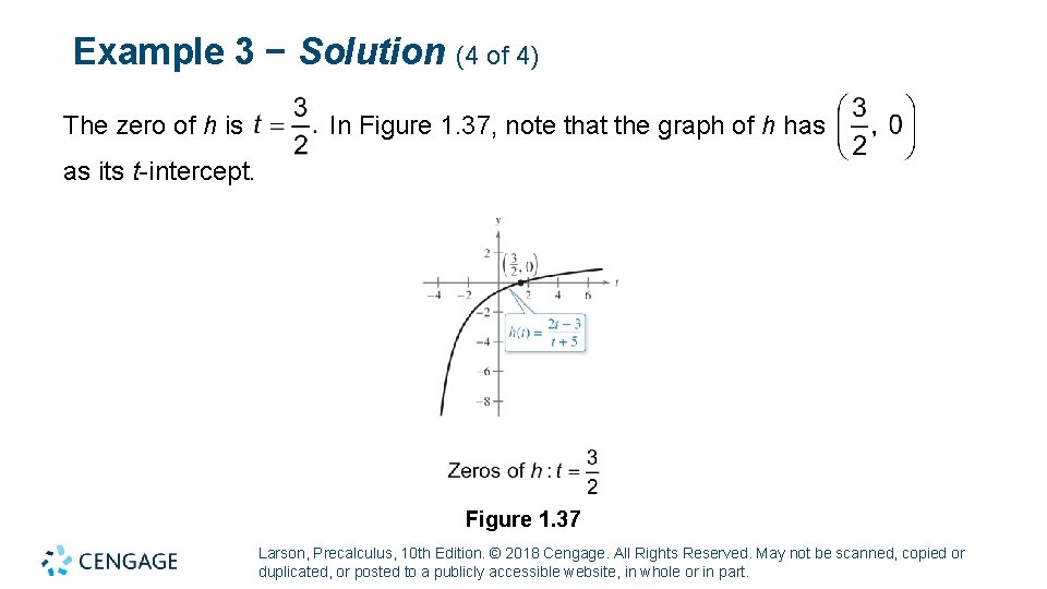
Example 3 − Solution (3 of 4) c. Set h(t) equal to 0. 2 t − 3 = 0 2 t = 3 Multiply each side by t + 5. Add 3 to each side. Divide each side by 2. Larson, Precalculus, 10 th Edition. © 2018 Cengage. All Rights Reserved. May not be scanned, copied or duplicated, or posted to a publicly accessible website, in whole or in part.

Example 3 − Solution (4 of 4) The zero of h is In Figure 1. 37, note that the graph of h has as its t -intercept. Figure 1. 37 Larson, Precalculus, 10 th Edition. © 2018 Cengage. All Rights Reserved. May not be scanned, copied or duplicated, or posted to a publicly accessible website, in whole or in part.

Increasing and Decreasing Functions Larson, Precalculus, 10 th Edition. © 2018 Cengage. All Rights Reserved. May not be scanned, copied or duplicated, or posted to a publicly accessible website, in whole or in part.

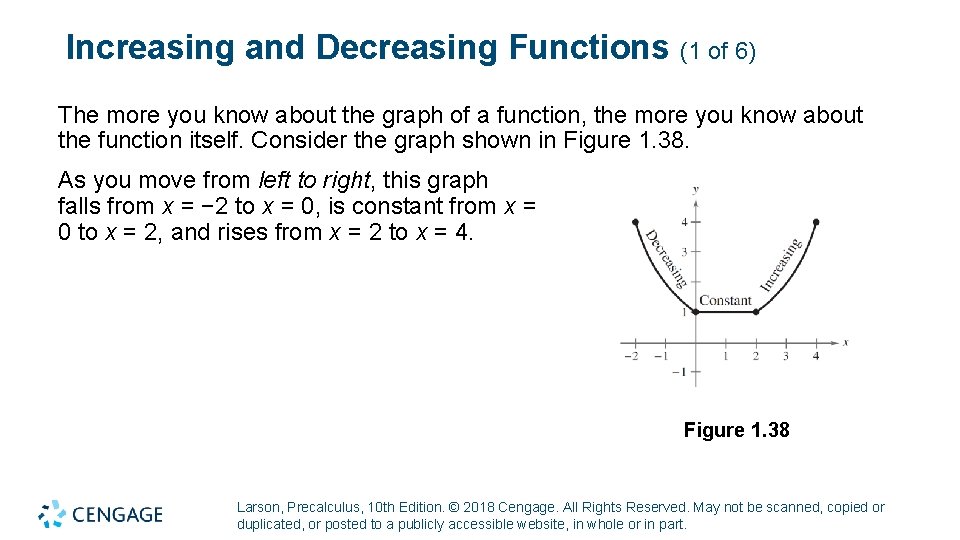
Increasing and Decreasing Functions (1 of 6) The more you know about the graph of a function, the more you know about the function itself. Consider the graph shown in Figure 1. 38. As you move from left to right, this graph falls from x = − 2 to x = 0, is constant from x = 0 to x = 2, and rises from x = 2 to x = 4. Figure 1. 38 Larson, Precalculus, 10 th Edition. © 2018 Cengage. All Rights Reserved. May not be scanned, copied or duplicated, or posted to a publicly accessible website, in whole or in part.

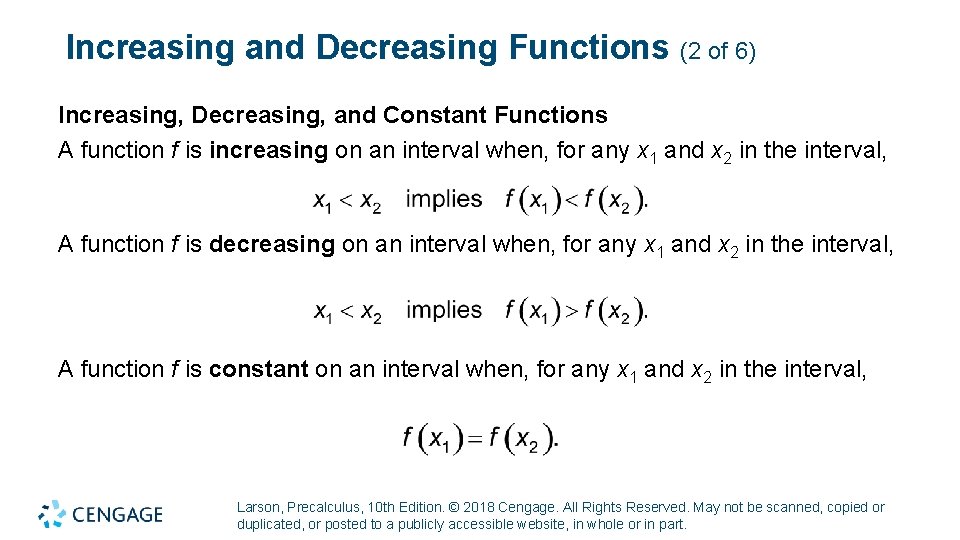
Increasing and Decreasing Functions (2 of 6) Increasing, Decreasing, and Constant Functions A function f is increasing on an interval when, for any x 1 and x 2 in the interval, A function f is decreasing on an interval when, for any x 1 and x 2 in the interval, A function f is constant on an interval when, for any x 1 and x 2 in the interval, Larson, Precalculus, 10 th Edition. © 2018 Cengage. All Rights Reserved. May not be scanned, copied or duplicated, or posted to a publicly accessible website, in whole or in part.

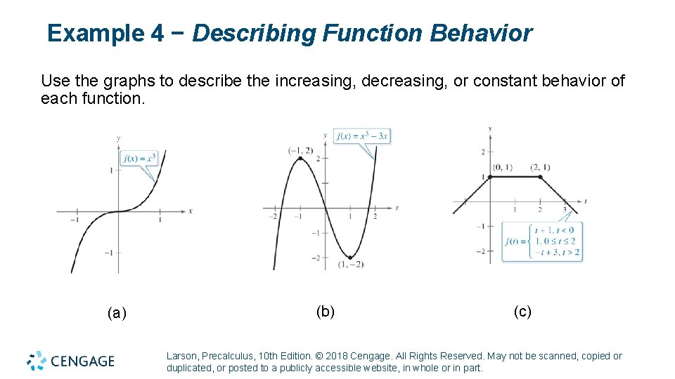
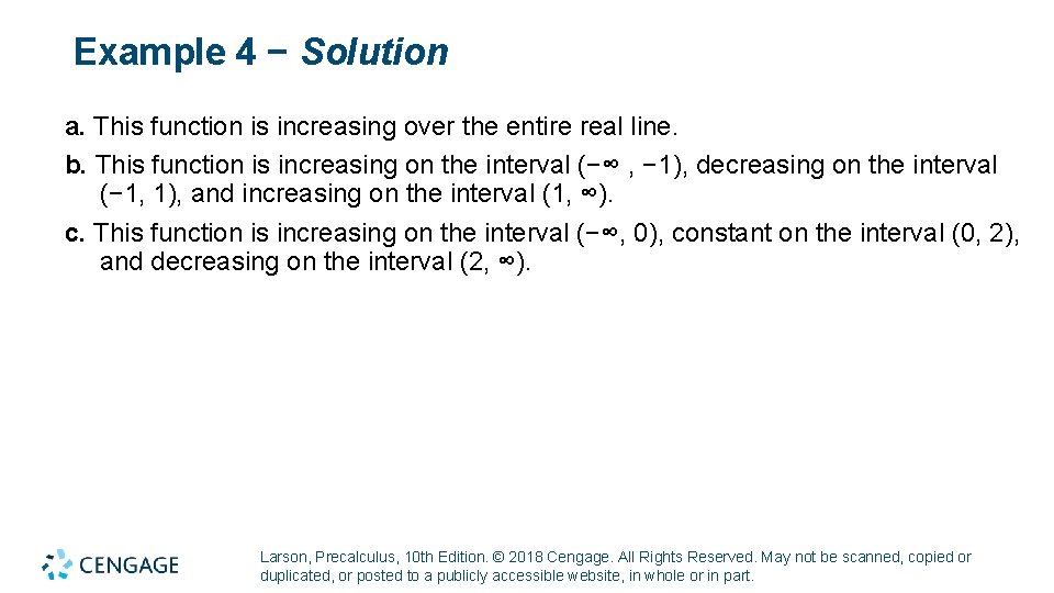
Example 4 − Describing Function Behavior Use the graphs to describe the increasing, decreasing, or constant behavior of each function. (a) (b) (c) Larson, Precalculus, 10 th Edition. © 2018 Cengage. All Rights Reserved. May not be scanned, copied or duplicated, or posted to a publicly accessible website, in whole or in part.

Example 4 − Solution a. This function is increasing over the entire real line. b. This function is increasing on the interval (−∞ , − 1), decreasing on the interval (− 1, 1), and increasing on the interval (1, ∞). c. This function is increasing on the interval (−∞, 0), constant on the interval (0, 2), and decreasing on the interval (2, ∞). Larson, Precalculus, 10 th Edition. © 2018 Cengage. All Rights Reserved. May not be scanned, copied or duplicated, or posted to a publicly accessible website, in whole or in part.

Increasing and Decreasing Functions (3 of 6) To help you decide whether a function is increasing, decreasing, or constant on an interval, you can evaluate the function for several values of x. However, you need calculus to determine, for certain, all intervals on which a function is increasing, decreasing, or constant. Larson, Precalculus, 10 th Edition. © 2018 Cengage. All Rights Reserved. May not be scanned, copied or duplicated, or posted to a publicly accessible website, in whole or in part.

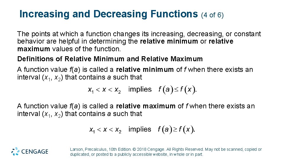
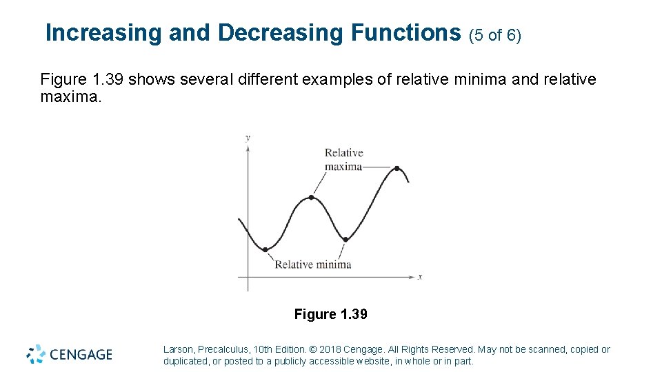
Increasing and Decreasing Functions (4 of 6) The points at which a function changes its increasing, decreasing, or constant behavior are helpful in determining the relative minimum or relative maximum values of the function. Definitions of Relative Minimum and Relative Maximum A function value f(a) is called a relative minimum of f when there exists an interval (x 1, x 2) that contains a such that A function value f(a) is called a relative maximum of f when there exists an interval (x 1, x 2) that contains a such that Larson, Precalculus, 10 th Edition. © 2018 Cengage. All Rights Reserved. May not be scanned, copied or duplicated, or posted to a publicly accessible website, in whole or in part.

Increasing and Decreasing Functions (5 of 6) Figure 1. 39 shows several different examples of relative minima and relative maxima. Figure 1. 39 Larson, Precalculus, 10 th Edition. © 2018 Cengage. All Rights Reserved. May not be scanned, copied or duplicated, or posted to a publicly accessible website, in whole or in part.

Increasing and Decreasing Functions (6 of 6) You will study a technique for finding the exact point at which a second-degree polynomial function has a relative minimum or relative maximum. For the time being, however, you can use a graphing utility to find reasonable approximations of these points. Larson, Precalculus, 10 th Edition. © 2018 Cengage. All Rights Reserved. May not be scanned, copied or duplicated, or posted to a publicly accessible website, in whole or in part.

Average Rate of Change Larson, Precalculus, 10 th Edition. © 2018 Cengage. All Rights Reserved. May not be scanned, copied or duplicated, or posted to a publicly accessible website, in whole or in part.

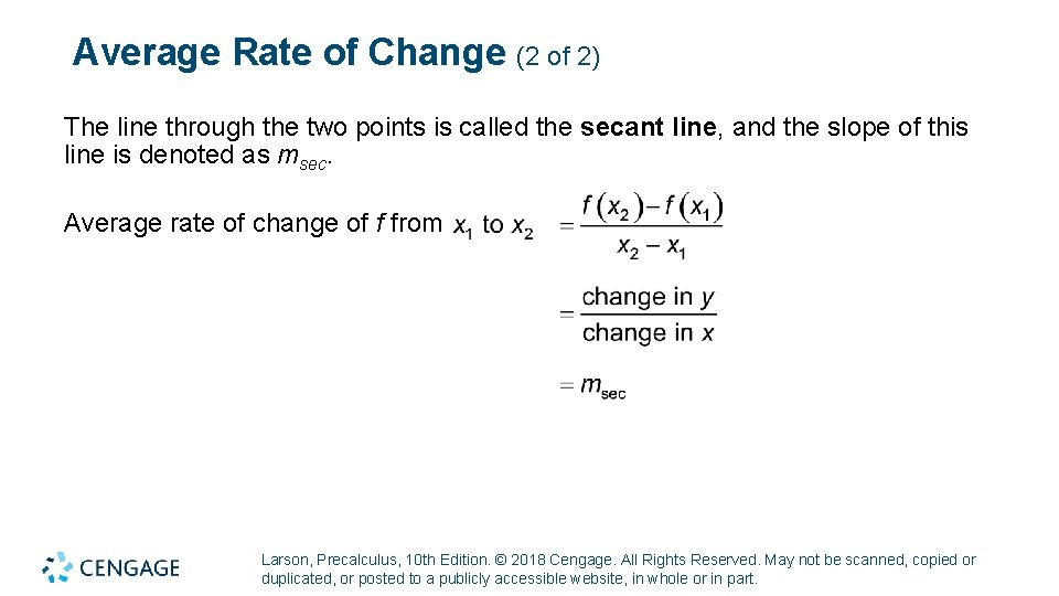
Average Rate of Change (1 of 2) We have learned that the slope of a line can be interpreted as a rate of change. For a nonlinear graph whose slope changes at each point, the average rate of change between any two points (x 1, f (x 1)) and (x 2, f (x 2)) is the slope of the line through the two points (see Figure 1. 41). Figure 1. 41 Larson, Precalculus, 10 th Edition. © 2018 Cengage. All Rights Reserved. May not be scanned, copied or duplicated, or posted to a publicly accessible website, in whole or in part.

Average Rate of Change (2 of 2) The line through the two points is called the secant line, and the slope of this line is denoted as msec. Average rate of change of f from Larson, Precalculus, 10 th Edition. © 2018 Cengage. All Rights Reserved. May not be scanned, copied or duplicated, or posted to a publicly accessible website, in whole or in part.

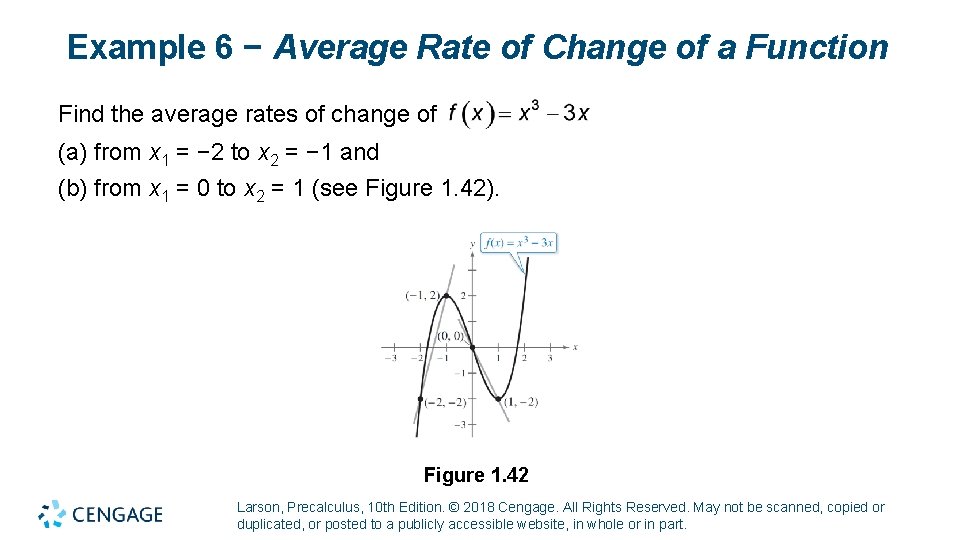
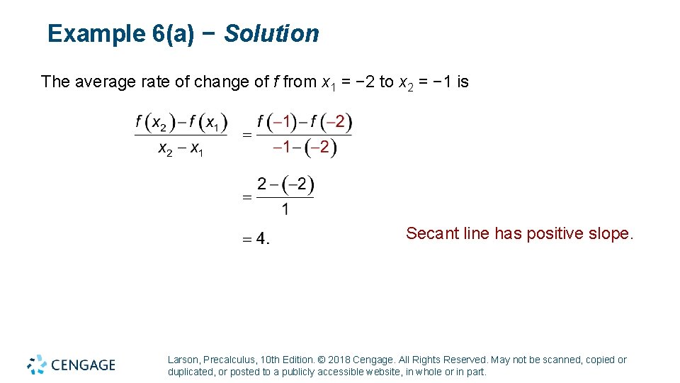
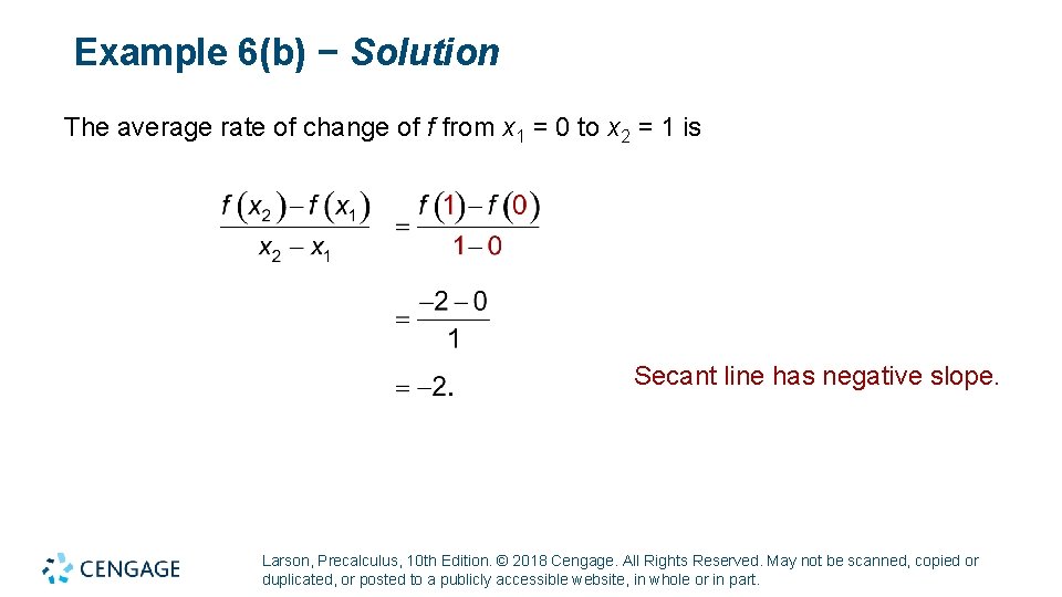
Example 6 − Average Rate of Change of a Function Find the average rates of change of (a) from x 1 = − 2 to x 2 = − 1 and (b) from x 1 = 0 to x 2 = 1 (see Figure 1. 42). Figure 1. 42 Larson, Precalculus, 10 th Edition. © 2018 Cengage. All Rights Reserved. May not be scanned, copied or duplicated, or posted to a publicly accessible website, in whole or in part.

Example 6(a) − Solution The average rate of change of f from x 1 = − 2 to x 2 = − 1 is Secant line has positive slope. Larson, Precalculus, 10 th Edition. © 2018 Cengage. All Rights Reserved. May not be scanned, copied or duplicated, or posted to a publicly accessible website, in whole or in part.

Example 6(b) − Solution The average rate of change of f from x 1 = 0 to x 2 = 1 is Secant line has negative slope. Larson, Precalculus, 10 th Edition. © 2018 Cengage. All Rights Reserved. May not be scanned, copied or duplicated, or posted to a publicly accessible website, in whole or in part.

Even and Odd Functions Larson, Precalculus, 10 th Edition. © 2018 Cengage. All Rights Reserved. May not be scanned, copied or duplicated, or posted to a publicly accessible website, in whole or in part.

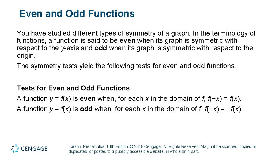
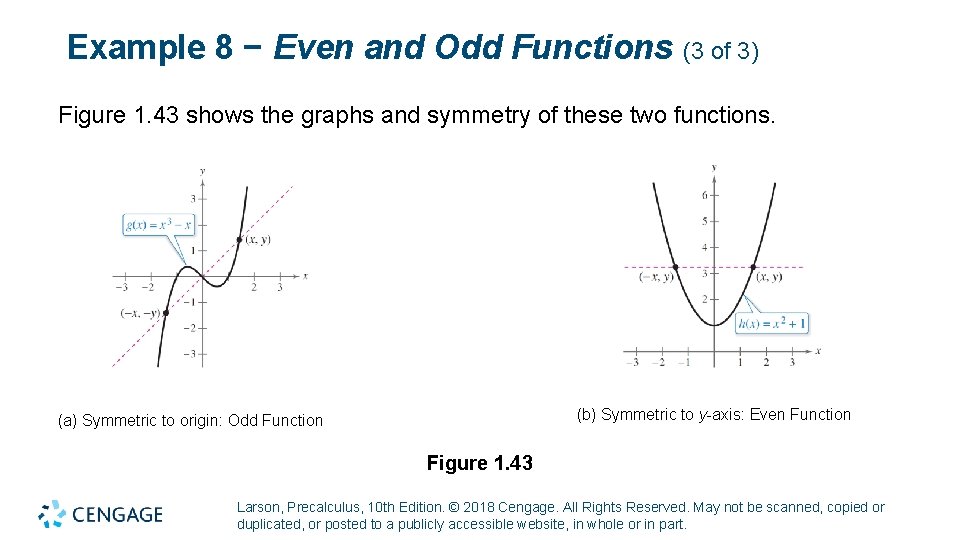
Even and Odd Functions You have studied different types of symmetry of a graph. In the terminology of functions, a function is said to be even when its graph is symmetric with respect to the y-axis and odd when its graph is symmetric with respect to the origin. The symmetry tests yield the following tests for even and odd functions. Tests for Even and Odd Functions A function y = f(x) is even when, for each x in the domain of f, f(−x) = f(x). A function y = f(x) is odd when, for each x in the domain of f, f(−x) = −f(x). Larson, Precalculus, 10 th Edition. © 2018 Cengage. All Rights Reserved. May not be scanned, copied or duplicated, or posted to a publicly accessible website, in whole or in part.

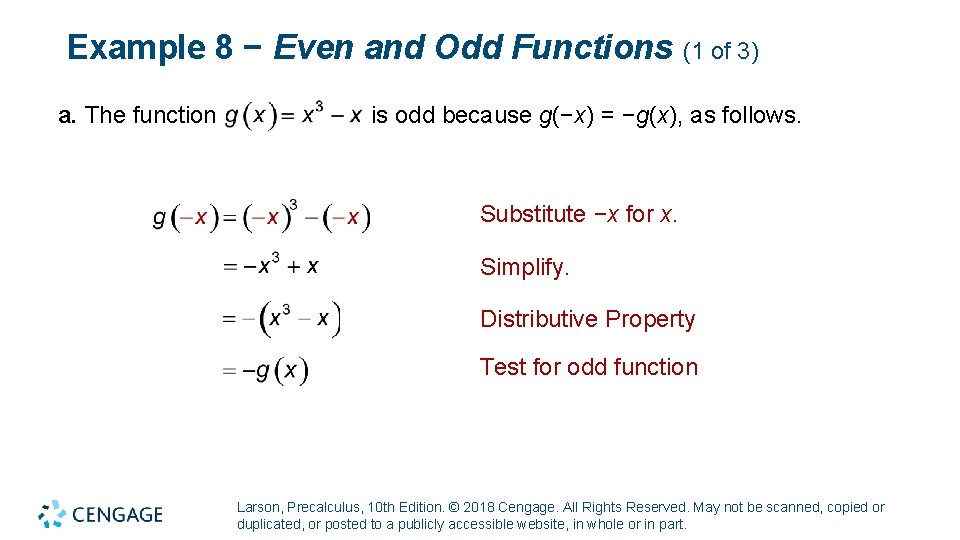
Example 8 − Even and Odd Functions (1 of 3) a. The function is odd because g(−x) = −g(x), as follows. Substitute −x for x. Simplify. Distributive Property Test for odd function Larson, Precalculus, 10 th Edition. © 2018 Cengage. All Rights Reserved. May not be scanned, copied or duplicated, or posted to a publicly accessible website, in whole or in part.

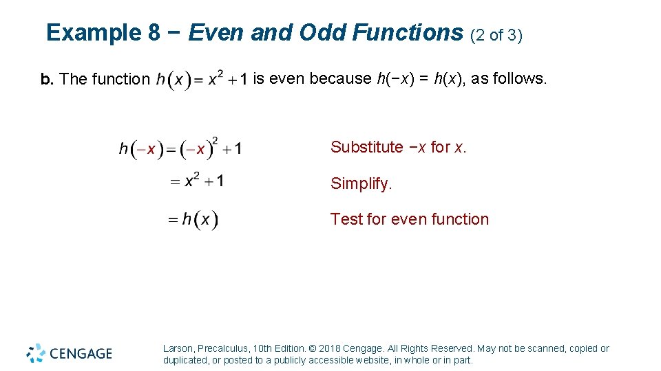
Example 8 − Even and Odd Functions (2 of 3) b. The function is even because h(−x) = h(x), as follows. Substitute −x for x. Simplify. Test for even function Larson, Precalculus, 10 th Edition. © 2018 Cengage. All Rights Reserved. May not be scanned, copied or duplicated, or posted to a publicly accessible website, in whole or in part.

Example 8 − Even and Odd Functions (3 of 3) Figure 1. 43 shows the graphs and symmetry of these two functions. (b) Symmetric to y-axis: Even Function (a) Symmetric to origin: Odd Function Figure 1. 43 Larson, Precalculus, 10 th Edition. © 2018 Cengage. All Rights Reserved. May not be scanned, copied or duplicated, or posted to a publicly accessible website, in whole or in part.