Chapter 1 Exploring Data Section 1 3 Describing

+ Chapter 1: Exploring Data Section 1. 3 Describing Quantitative Data with Numbers The Practice of Statistics, 4 th edition - For AP* STARNES, YATES, MOORE

+ Chapter 1 Exploring Data n Introduction: Data Analysis: Making Sense of Data n 1. 1 Analyzing Categorical Data n 1. 2 Displaying Quantitative Data with Graphs n 1. 3 Describing Quantitative Data with Numbers

+ Section 1. 3 Describing Quantitative Data with Numbers Learning Objectives After this section, you should be able to… ü MEASURE center with the mean and median ü MEASURE spread with standard deviation and interquartile range ü IDENTIFY outliers ü CONSTRUCT a boxplot using the five-number summary ü CALCULATE numerical summaries with technology

The most common measure of center is the ordinary arithmetic average, or mean. Definition: To find the mean (pronounced “x-bar”) of a set of observations, add their values and divide by the number of observations. If the n observations are x 1, x 2, x 3, …, xn, their mean is: In mathematics, the capital Greek letter Σis short for “add them all up. ” Therefore, the formula for the mean can be written in more compact notation: Describing Quantitative Data n Center: The Mean + n Measuring

Example 1: Here is a stemplot of the travel times to work for the sample of 15 North Carolinians. a) Find the mean travel time for all 15 workers.

b) Calculate the mean again, this time excluding the person who reported a 60 -minute travel time to work. What do you notice? This one observation raises the mean by 2. 7 minutes.

Comparing the Mean and the Median Our discussion of travel times to work in North Carolina illustrates an important difference between the mean and the median. The median travel time (the midpoint of the distribution) is 20 minutes. The mean travel time is higher, 22. 5 minutes. The mean is pulled toward the right tail of this right-skewed distribution. The median, unlike the mean, is resistant. If the longest travel time were 600 minutes rather than 60 minutes, the mean would increase to more than 58 minutes but the median would not change at all. The outlier just counts as one observation above the center, no matter how far above the center it lies. The mean uses the actual value of each observation and so will chase a single large observation upward.

Another common measure of center is the median. In section 1. 2, we learned that the median describes the midpoint of a distribution. Definition: The median M is the midpoint of a distribution, the number such that half of the observations are smaller and the other half are larger. To find the median of a distribution: 1)Arrange all observations from smallest to largest. 2)If the number of observations n is odd, the median M is the center observation in the ordered list. 3)If the number of observations n is even, the median M is the average of the two center observations in the ordered list. Describing Quantitative Data n Center: The Median + n Measuring

Use the data below to calculate the mean and median of the commuting times (in minutes) of 20 randomly selected New York workers. Example, page 53 10 30 0 1 2 3 4 5 6 7 8 5 25 40 20 10 15 5 005555 0005 Key: 4|5 00 represents a 005 5 New York worker who reported a 45 minute travel time to work. 30 20 15 20 85 15 60 60 40 45 Describing Quantitative Data n Center + n Measuring

n The mean and median measure center in different ways, and both are useful. n Don’t confuse the “average” value of a variable (the mean) with its “typical” value, which we might describe by the median. Comparing the Mean and the Median The mean and median of a roughly symmetric distribution are close together. If the distribution is exactly symmetric, the mean and median are exactly the same. In a skewed distribution, the mean is usually farther out in the long tail than is the median. + Comparing the Mean and the Median Describing Quantitative Data n

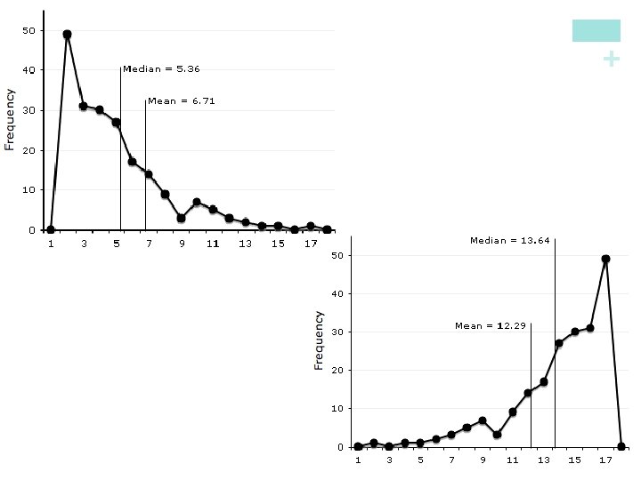
+ Why is the mean more affected by the presence of outliers than the median?

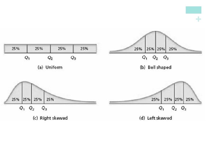
Spread: The Interquartile Range (IQR) A measure of center alone can be misleading. n A useful numerical description of a distribution requires both a measure of center and a measure of spread. How to Calculate the Quartiles and the Interquartile Range To calculate the quartiles: 1)Arrange the observations in increasing order and locate the median M. 2)The first quartile Q 1 is the median of the observations located to the left of the median in the ordered list. 3)The third quartile Q 3 is the median of the observations located to the right of the median in the ordered list. The interquartile range (IQR) is defined as: IQR = Q 3 – Q 1 Describing Quantitative Data n + n Measuring

+ Interquartile Range (IQR)

and Interpret the IQR + n Find 10 30 5 25 40 20 10 15 30 20 15 20 85 15 60 60 40 45 5 10 10 15 15 20 20 20 25 30 30 40 40 45 60 60 65 85 Q 1 = 15 M = 22. 5 Q 3= 42. 5 IQR = Q 3 – Q 1 = 42. 5 – 15 = 27. 5 minutes Interpretation: The range of the middle half of travel times for the New Yorkers in the sample is 27. 5 minutes. Describing Quantitative Data Travel times to work for 20 randomly selected New Yorkers

In addition to serving as a measure of spread, the interquartile range (IQR) is used as part of a rule of thumb for identifying outliers. Definition: The 1. 5 x IQR Rule for Outliers Call an observation an outlier if it falls more than 1. 5 x IQR above third quartile or below the first quartile. In the New York travel time data, we found Q 1=15 minutes, Q 3=42. 5 minutes, and IQR=27. 5 minutes. 0 1 2 For these data, 1. 5 x IQR = 1. 5(27. 5) = 41. 25 3 Q 1 - 1. 5 x IQR = 15 – 41. 25 = -26. 25 4 Q 3+ 1. 5 x IQR = 42. 5 + 41. 25 = 83. 75 5 Any travel time shorter than -26. 25 minutes or longer than 6 7 83. 75 minutes is considered an outlier. 8 5 005555 0005 00 005 5 Describing Quantitative Data n Outliers + n Identifying

+ AP EXAM TIP n. You may be asked to determine whether a quantitative data set has any outliers. Be prepared to state and use the rule for identifying outliers.

+ Five-Number Summary n The minimum and maximum values alone tell us little about the distribution as a whole. Likewise, the median and quartiles tell us little about the tails of a distribution. n To get a quick summary of both center and spread, combine all five numbers. Definition: The five-number summary of a distribution consists of the smallest observation, the first quartile, the median, the third quartile, and the largest observation, written in order from smallest to largest. Minimum Q 1 M Q 3 Maximum Describing Quantitative Data n The

• Draw and label a number line that includes the range of the distribution. • Draw a central box from Q 1 to Q 3. • Note the median M inside the box. • Extend lines (whiskers) from the box out to the minimum and maximum values that are not outliers. + Boxplots (Box-and-Whisker Plots)

a Boxplot + n Construct Consider our NY travel times data. Construct a boxplot. n 10 30 5 25 40 20 10 15 30 20 15 20 85 15 60 60 40 45 5 10 10 15 15 20 20 20 25 30 30 40 40 45 60 60 65 85 Min=5 Q 1 = 15 M = 22. 5 Q 3= 42. 5 Max=85 Recall, this is an outlier by the 1. 5 x IQR rule Describing Quantitative Data Example

n The most common measure of spread looks at how far each observation is from the mean. This measure is called the standard deviation. Let’s explore it! Consider the following data on the number of pets owned by a group of 9 children. 1) Calculate the mean. 2) Calculate each deviation = observation – mean deviation: 1 - 5 = -4 deviation: 8 - 5 = 3 =5 Describing Quantitative Data n Spread: The Standard Deviation + n Measuring

Spread: The Standard Deviation 4) Find the “average” squared deviation. Calculate the sum of the squared deviations divided by (n-1)…this is called the variance. 5) Calculate the square root of the variance…this is the standard deviation. (xi-mean) 1 1 - 5 = -4 (-4)2 = 16 3 3 - 5 = -2 (-2)2 = 4 4 4 - 5 = -1 (-1)2 = 1 5 5 -5=0 (0)2 = 0 7 7 -5=2 (2)2 = 4 8 8 -5=3 (3)2 = 9 9 9 -5=4 (4)2 = 16 Sum=? “average” squared deviation = 52/(9 -1) = 6. 5 Standard deviation = square root of variance = (xi-mean)2 Describing Quantitative Data 3) Square each deviation. xi + n Measuring Sum=? This is the variance.

Spread: The Standard Deviation Definition: The standard deviation sx measures the average distance of the observations from their mean. It is calculated by finding an average of the squared distances and then taking the square root. This average squared distance is called the variance. + n Measuring

+ Standard Deviation n. A relatively low standard deviation value indicates that the data points tend to be very close to the mean. n. A relatively high standard deviation value indicates that the data points are spread out over a large range of values.

+ Two Extreme Examples: n In dataset #1, we have five people that report eating 4 pieces of cake and five people that report eating 6 pieces of cake, for a mean of 5 pieces of cake ([4+4+4+6+6+6]/10=5). n Mean n =5; Variance = 1 In dataset #2, we have five people that report eating 0 piece of cake and five people that report eating 10 pieces of cake, for a mean of 5 pieces of cake ([0+0+0+10+10+10]/10=5). n Mean = 5; Variance = 5

+ Below are dotplots of three different distributions, A, B, and C. Which one has the largest standard deviation? Justify your answer.

n We now have a choice between two descriptions for center and spread n Mean and Standard Deviation n Median and Interquartile Range Choosing Measures of Center and Spread • The median and IQR are usually better than the mean and standard deviation for describing a skewed distribution or a distribution with outliers. • Use mean and standard deviation only for reasonably symmetric distributions that don’t have outliers. • NOTE: Numerical summaries do not fully describe the shape of a distribution. ALWAYS PLOT YOUR DATA! + Choosing Measures of Center and Spread Describing Quantitative Data n

+ AP EXAM TIP n. Use statistical terms carefully and correctly on the AP exam. Don’t say “mean” if you really mean “median. ” Range is a single number; so are Q 1, Q 3, and IQR. Avoid colloquial use of language, like “the outlier skews the mean. ” Skewed is a shape. If you misuse a term, expect to lose some credit.

Organizing a Statistical Problem As you learn more about statistics, you will be asked to solve more complex problems. Here is a four-step process you can follow. How to Organize a Statistical Problem: A Four-Step Process State: What’s the question that you’re trying to answer? Plan: How will you go about answering the question? What statistical techniques does this problem call for? Do: Make graphs and carry out needed calculations. Conclude: Give your conclusion in the setting of the real-world problem.

Example 7: For their final project, a group of AP Statistics students wanted to compare the texting habits of males and female. They asked a random sample of students from their school to record the number of text messages sent and received over a two-day period. Here are their data: What conclusion should the students draw? Give appropriate evidence to support your answer. Do males and females at the school differ in their texting habits? STATE: Do males and females at the school differ in their texting habits. PLAN: We’ll begin by making parallel boxplots of the data about males and females. Then we’ll calculate one-variable statistics. Finally, we’ll compare shape, center, spread, and outliers for the two distributions.

DO: The figure below is a sketch of the boxplots we got from our calculator. The table below shows numerical summaries for males and females.

Due to the strong skewness and outliers, we’ll use the median and IQR instead of the mean and standard deviation when comparing center and spread. Shape: Both distributions are strongly right-skewed. Center: Females typically text more than males. The median number of texts for females (107) is about four times as high as for males (28). In fact, the median for the females is above third quartile for the males. This indicates that over 75% of the males texted less than the “typical” (median) female. Spread: There is much more variation in texting among the females than the males. The IQR for females (157) is about twice the IQR for males (77). Outliers: There are two outliers in the male distribution: students who reported 213 and 214 texts in two days. The female distribution has no outliers.

CONCLUDE: The data from this survey project give very strong evidence that male and female texting habits differ considerably at the school. A typical female sends and receives about 79 more text messages in a two-day period than a typical male. The males as a group are also much more consistent in their texting frequency than the females.

+ FRQ 2018 #5

Symmetric Distribution Best Measure of Center Best Measure of Spread Skewed Distribution + Choosing Best Measures of Center & Spread

+ Section 1. 3 Describing Quantitative Data with Numbers Summary In this section, we learned that… ü A numerical summary of a distribution should report at least its center and spread. ü The mean and median describe the center of a distribution in different ways. The mean is the average and the median is the midpoint of the values. ü When you use the median to indicate the center of a distribution, describe its spread using the quartiles. ü The interquartile range (IQR) is the range of the middle 50% of the observations: IQR = Q 3 – Q 1.

+ Section 1. 3 Describing Quantitative Data with Numbers Summary In this section, we learned that… ü An extreme observation is an outlier if it is smaller than –(1. 5 x. IQR) or larger than Q 3+(1. 5 x. IQR). Q 1 ü The five-number summary (min, Q 1, M, Q 3, max) provides a quick overall description of distribution and can be pictured using a boxplot. ü The variance and its square root, the standard deviation are common measures of spread about the mean as center. ü The mean and standard deviation are good descriptions for symmetric distributions without outliers. The median and IQR are a better description for skewed distributions.

+ Looking Ahead… In the next Chapter… We’ll learn how to model distributions of data… • Describing Location in a Distribution • Normal Distributions