Chapter 1 Exploring Data Section 1 3 Describing

+ Chapter 1: Exploring Data Section 1. 3 Describing Quantitative Data with Numbers The Practice of Statistics, 4 th edition - For AP* STARNES, YATES, MOORE

+ Chapter 1 Exploring Data n Introduction: Data Analysis: Making Sense of Data n 1. 1 Analyzing Categorical Data n 1. 2 Displaying Quantitative Data with Graphs n 1. 3 Describing Quantitative Data with Numbers

+ Section 1. 3 Describing Quantitative Data with Numbers Learning Objectives After this section, you should be able to… ü MEASURE center with the mean and median ü MEASURE spread with standard deviation and interquartile range ü IDENTIFY outliers ü CONSTRUCT a boxplot using the five-number summary ü CALCULATE numerical summaries with technology

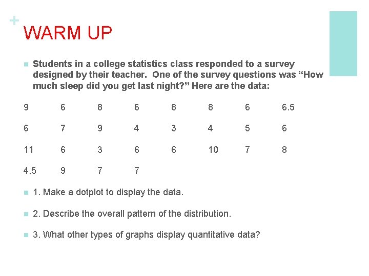
+ WARM UP n Students in a college statistics class responded to a survey designed by their teacher. One of the survey questions was “How much sleep did you get last night? ” Here are the data: 9 6 8 8 6 6. 5 6 7 9 4 3 4 5 6 11 6 3 6 6 10 7 8 4. 5 9 7 7 n 1. Make a dotplot to display the data. n 2. Describe the overall pattern of the distribution. n 3. What other types of graphs display quantitative data?

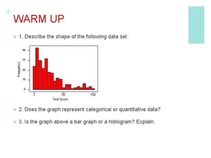
+ WARM UP n 1. Describe the shape of the following data set. n 2. Does the graph represent categorical or quantitative data? n 3. Is the graph above a bar graph or a histogram? Explain.

n Examples: “all women in the Bay Area between the ages of 18 and 54. ” “House cats raised as pets in American households. ” “The light bulbs we are manufacturing in this plant. ” Sample: A sample is a group of units selected from a larger group (the population). By studying the sample it is hoped to draw valid conclusions about the larger group. n Examples: “ 500 women in the Bay Area between the ages of 18 and 54. ” “ 50 house cats drawn from households in San Francisco, CA. ” “ 10 light bulbs manufactured at this plant in the last year. ” + Population Parameters vs. Sample Statistics Population: A population is any entire collection of people, animals, plants or things from which we may collect data. It is the entire group we are interested in, which we wish to describe or draw conclusions about.

n Statistic: A statistic is a quantity that is calculated from a sample of data. It is used to give information about unknown values in the corresponding population. Population Parameters vs. Sample Statistics A parameter is a value, usually unknown (and which therefore has to be estimated), used to represent a certain population characteristic. + n Parameter:

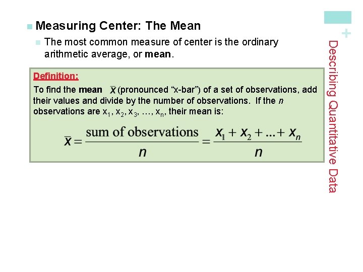
The most common measure of center is the ordinary arithmetic average, or mean. Definition: To find the mean (pronounced “x-bar”) of a set of observations, add their values and divide by the number of observations. If the n observations are x 1, x 2, x 3, …, xn, their mean is: Describing Quantitative Data n Center: The Mean + n Measuring

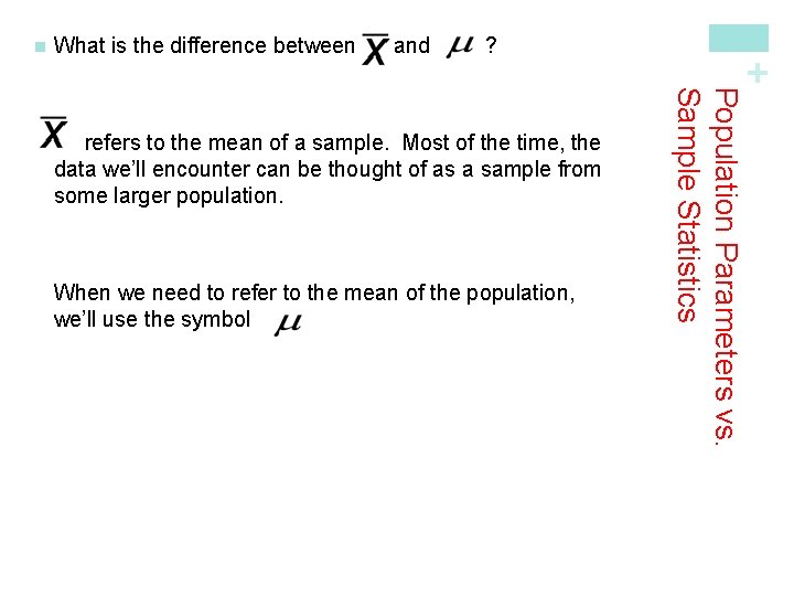
What is the difference between and ? + n When we need to refer to the mean of the population, we’ll use the symbol Population Parameters vs. Sample Statistics refers to the mean of a sample. Most of the time, the data we’ll encounter can be thought of as a sample from some larger population.

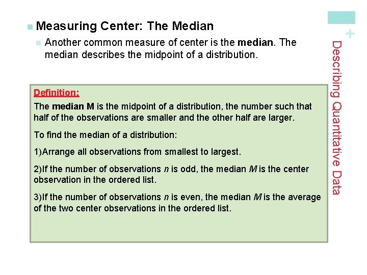
Another common measure of center is the median. The median describes the midpoint of a distribution. Definition: The median M is the midpoint of a distribution, the number such that half of the observations are smaller and the other half are larger. To find the median of a distribution: 1)Arrange all observations from smallest to largest. 2)If the number of observations n is odd, the median M is the center observation in the ordered list. 3)If the number of observations n is even, the median M is the average of the two center observations in the ordered list. Describing Quantitative Data n Center: The Median + n Measuring

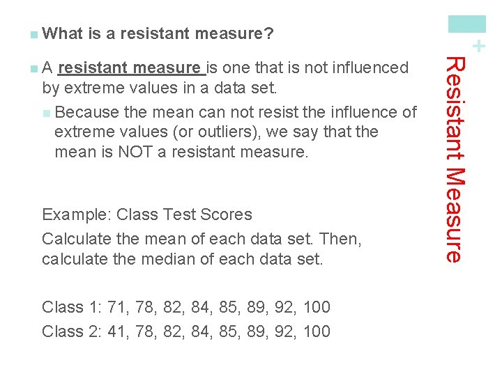
is a resistant measure? resistant measure is one that is not influenced by extreme values in a data set. n Because the mean can not resist the influence of extreme values (or outliers), we say that the mean is NOT a resistant measure. Example: Class Test Scores Calculate the mean of each data set. Then, calculate the median of each data set. Class 1: 71, 78, 82, 84, 85, 89, 92, 100 Class 2: 41, 78, 82, 84, 85, 89, 92, 100 Resistant Measure n. A + n What

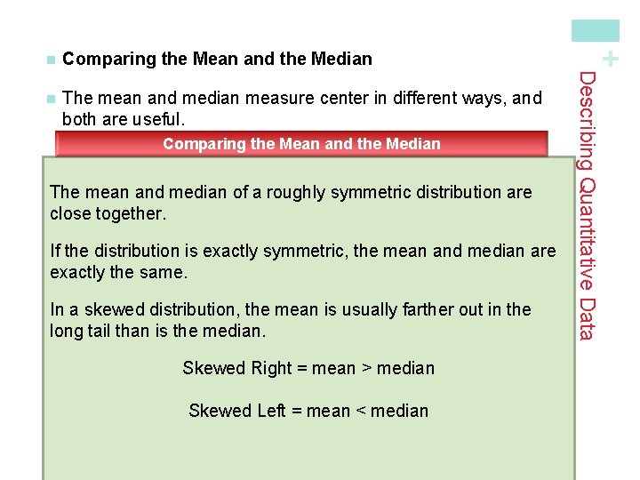
n The mean and median measure center in different ways, and both are useful. Comparing the Mean and the Median The mean and median of a roughly symmetric distribution are close together. If the distribution is exactly symmetric, the mean and median are exactly the same. In a skewed distribution, the mean is usually farther out in the long tail than is the median. Skewed Right = mean > median Skewed Left = mean < median + Comparing the Mean and the Median Describing Quantitative Data n

Spread A measure of center alone can be misleading. n A useful numerical description of a distribution requires both a measure of center and a measure of spread. Measures of Spread: • Range • IQR • Standard Deviation Describing Quantitative Data n + n Measuring

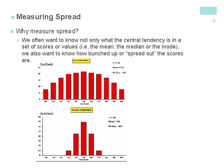
n Spread Why measure spread? n We often want to know not only what the central tendency is in a set of scores or values (i. e, the mean, the median or the mode), we also want to know how bunched up or “spread out” the scores are. + n Measuring

Spread: The Range The range is the difference between the highest value and the lowest value in a data set n Example: Class Test Scores Find the range of each class. 71, 78, 82, 84, 85, 89, 92, 100 41, 78, 82, 84, 85, 89, 92, 100 n Is the range a resistant measure? Describing Quantitative Data n + n Measuring

Spread: The Interquartile Range (IQR) The difference between the first and third quartiles in a data set n Before you can find the IQR, you need to find the quartiles How to Calculate the Quartiles and the Interquartile Range Quartiles: Points that divide the data set into 4 equal pieces ***Note: there are only 3 of them! 1)Arrange the observations in increasing order and locate the median M. 2)The first quartile Q 1 is the median of the observations located to the left of the median in the ordered list. 3)The third quartile Q 3 is the median of the observations located to the right of the median in the ordered list. The interquartile range (IQR) is defined as: IQR = Q 3 – Q 1 Describing Quantitative Data n + n Measuring

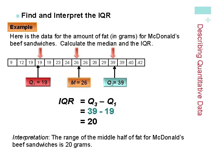
and Interpret the IQR + n Find Here is the data for the amount of fat (in grams) for Mc. Donald’s beef sandwiches. Calculate the median and the IQR. 9 12 19 19 19 Q 1 = 19 23 24 26 26 M = 26 28 29 39 39 40 42 Q 3= 39 IQR = Q 3 – Q 1 = 39 - 19 = 20 Interpretation: The range of the middle half of fat for Mc. Donald’s beef sandwiches is 20 grams. Describing Quantitative Data Example

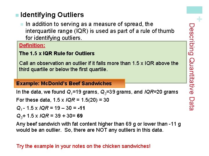
In addition to serving as a measure of spread, the interquartile range (IQR) is used as part of a rule of thumb for identifying outliers. Definition: The 1. 5 x IQR Rule for Outliers Call an observation an outlier if it falls more than 1. 5 x IQR above third quartile or below the first quartile. Example: Mc. Donld’s Beef Sandwiches In the data, we found Q 1=19 grams, Q 3=39 grams, and IQR=20 grams For these data, 1. 5 x IQR = 1. 5(20) = 30 Q 1 - 1. 5 x IQR = 19 – 30 = -11 Q 3+ 1. 5 x IQR = 39 + 30= 69 Any beef sandwich with fat content higher than 69 g or lower than -11 g would be an outlier. So, there are NOT any outliers in this data. Try the example in your notes on the chicken sandwiches! Describing Quantitative Data n Outliers + n Identifying

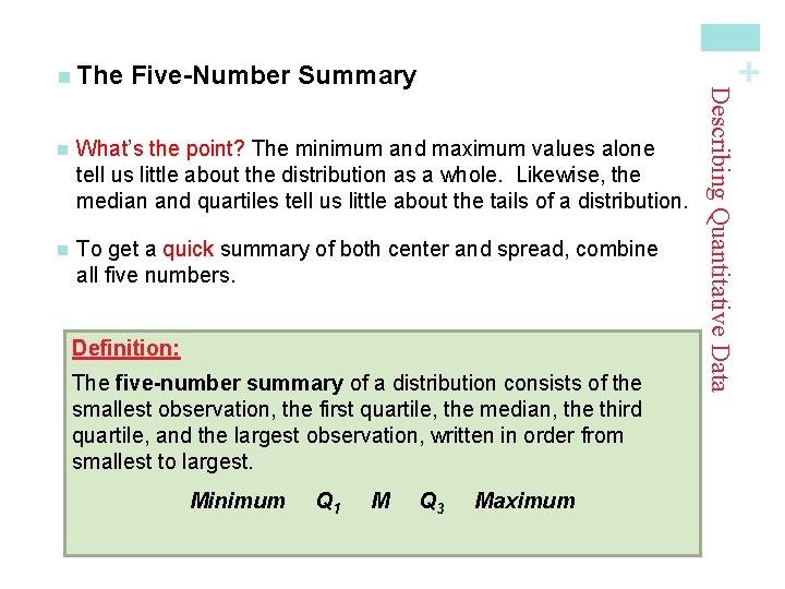
+ Five-Number Summary n What’s the point? The minimum and maximum values alone tell us little about the distribution as a whole. Likewise, the median and quartiles tell us little about the tails of a distribution. n To get a quick summary of both center and spread, combine all five numbers. Definition: The five-number summary of a distribution consists of the smallest observation, the first quartile, the median, the third quartile, and the largest observation, written in order from smallest to largest. Minimum Q 1 M Q 3 Maximum Describing Quantitative Data n The

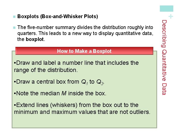
n The five-number summary divides the distribution roughly into quarters. This leads to a new way to display quantitative data, the boxplot. How to Make a Boxplot • Draw and label a number line that includes the range of the distribution. • Draw a central box from Q 1 to Q 3. • Note the median M inside the box. • Extend lines (whiskers) from the box out to the minimum and maximum values that are not outliers. + Boxplots (Box-and-Whisker Plots) Describing Quantitative Data n

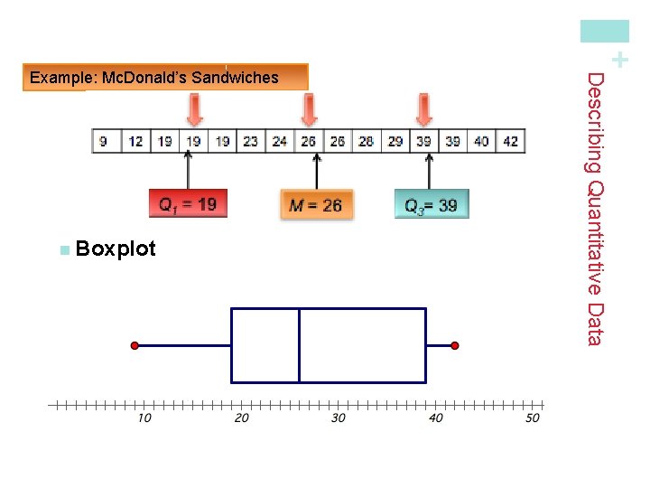
n Boxplot n Consider our beef sandwiches data. Construct a boxplot. + Describing Quantitative Data Example: Mc. Donald’s Sandwiches

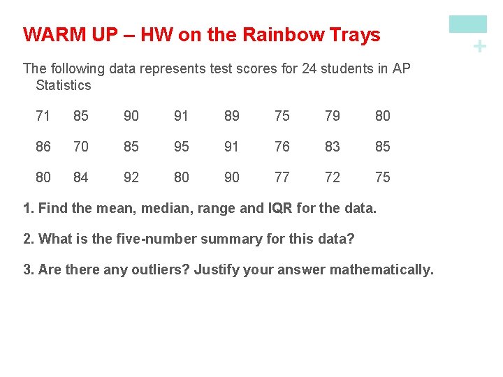
The following data represents test scores for 24 students in AP Statistics 71 85 90 91 89 75 79 80 86 70 85 95 91 76 83 85 80 84 92 80 90 77 72 75 1. Find the mean, median, range and IQR for the data. 2. What is the five-number summary for this data? 3. Are there any outliers? Justify your answer mathematically. + WARM UP – HW on the Rainbow Trays

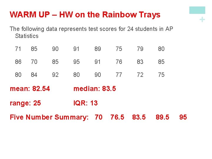
+ WARM UP – HW on the Rainbow Trays The following data represents test scores for 24 students in AP Statistics 71 85 90 91 89 75 79 80 86 70 85 95 91 76 83 85 80 84 92 80 90 77 72 75 83. 5 89. 5 mean: 82. 54 median: 83. 5 range: 25 IQR: 13 Five Number Summary: 70 76. 5 95

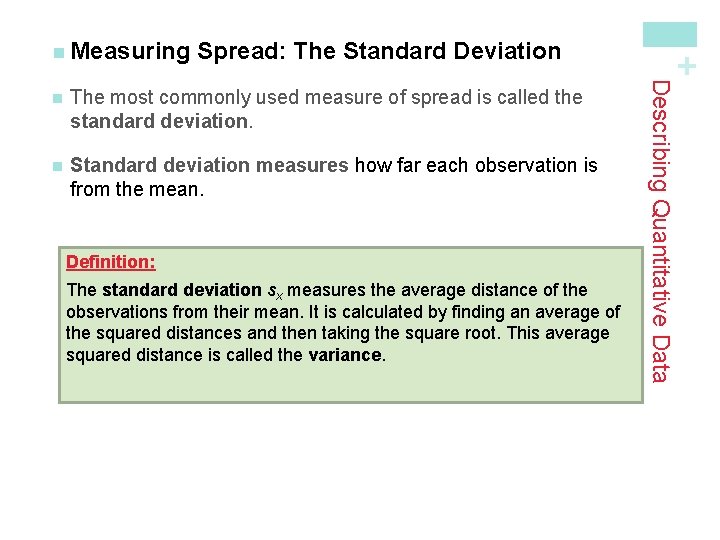
Spread: The Standard Deviation The most commonly used measure of spread is called the standard deviation. n Standard deviation measures how far each observation is from the mean. Definition: The standard deviation sx measures the average distance of the observations from their mean. It is calculated by finding an average of the squared distances and then taking the square root. This average squared distance is called the variance. Describing Quantitative Data n + n Measuring

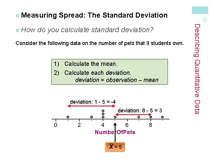
do you calculate standard deviation? Consider the following data on the number of pets that 9 students own. 1) Calculate the mean. 2) Calculate each deviation = observation – mean deviation: 1 - 5 = -4 deviation: 8 - 5 = 3 =5 Describing Quantitative Data n How Spread: The Standard Deviation + n Measuring

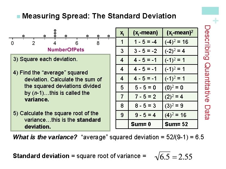
Spread: The Standard Deviation 4) Find the “average” squared deviation. Calculate the sum of the squared deviations divided by (n-1)…this is called the variance. 5) Calculate the square root of the variance…this is the standard deviation. (xi-mean) 1 1 - 5 = -4 (-4)2 = 16 3 3 - 5 = -2 (-2)2 = 4 4 4 - 5 = -1 (-1)2 = 1 5 5 -5=0 (0)2 = 0 7 7 -5=2 (2)2 = 4 8 8 -5=3 (3)2 = 9 9 9 -5=4 (4)2 = 16 Sum= 0 (xi-mean)2 Describing Quantitative Data 3) Square each deviation. xi + n Measuring Sum= 52 What is the variance? “average” squared deviation = 52/(9 -1) = 6. 5 Standard deviation = square root of variance =

What are the similarities and differences between range, IQR and standard deviation? n Similarities: all are measures of variability n Differences: resistance to outliers, using all of the data n What are some properties of standard deviation? n Standard deviation is never negative. n Standard deviation is sensitive to outliers. A single outlier can raise the standard deviation and in turn, distort the picture of spread. n For data with approximately the same mean, the greater the spread, the greater the standard deviation. n If all values of a data set are the same, the standard deviation is zero (because each value is equal to the mean). + n

Standard Deviation A random sample of 5 students was asked how many minutes they spent doing homework the previous night. Here are there responses (in minutes): 0, 25, 30, 60, 90. Calculate and interpret the standard deviation. + n Example:

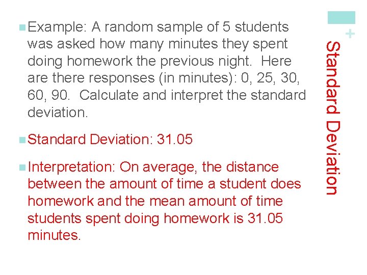
n Standard Deviation: 31. 05 n Interpretation: On average, the distance between the amount of time a student does homework and the mean amount of time students spent doing homework is 31. 05 minutes. Standard Deviation A random sample of 5 students was asked how many minutes they spent doing homework the previous night. Here are there responses (in minutes): 0, 25, 30, 60, 90. Calculate and interpret the standard deviation. + n Example:

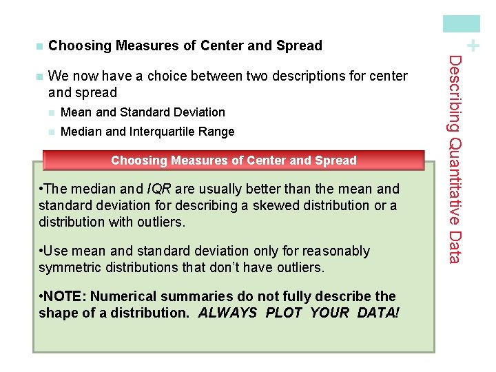
n We now have a choice between two descriptions for center and spread n Mean and Standard Deviation n Median and Interquartile Range Choosing Measures of Center and Spread • The median and IQR are usually better than the mean and standard deviation for describing a skewed distribution or a distribution with outliers. • Use mean and standard deviation only for reasonably symmetric distributions that don’t have outliers. • NOTE: Numerical summaries do not fully describe the shape of a distribution. ALWAYS PLOT YOUR DATA! + Choosing Measures of Center and Spread Describing Quantitative Data n

+ Section 1. 3 Describing Quantitative Data with Numbers Summary In this section, we learned that… ü A numerical summary of a distribution should report at least its center and spread. ü The mean and median describe the center of a distribution in different ways. The mean is the average and the median is the midpoint of the values. ü When you use the median to indicate the center of a distribution, describe its spread using the quartiles. ü The interquartile range (IQR) is the range of the middle 50% of the observations: IQR = Q 3 – Q 1.

+ Section 1. 3 Describing Quantitative Data with Numbers Summary In this section, we learned that… ü An extreme observation is an outlier if it is smaller than –(1. 5 x. IQR) or larger than Q 3+(1. 5 x. IQR). Q 1 ü The five-number summary (min, Q 1, M, Q 3, max) provides a quick overall description of distribution and can be pictured using a boxplot. ü The variance and its square root, the standard deviation are common measures of spread about the mean as center. ü The mean and standard deviation are good descriptions for symmetric distributions without outliers. The median and IQR are a better description for skewed distributions.

+ Looking Ahead… In the next Chapter… We’ll learn how to model distributions of data… • Describing Location in a Distribution • Normal Distributions