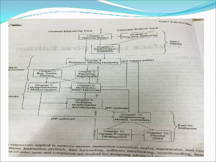
Chapter 1 Elements of a modern computer Elements

Chapter 1

Elements of a modern computer

Elements of a modern computer Computing problems: the problems for which computer system should be constructed. Algorithms and data structure: Special algorithms and data structures are needed to specify the computations and communications involved in computing problems. Hardware resources: Processors, memory, peripheral devices.

Operating system: System software support: Programs written in High level language. The source code translated into object code by a compiler. • Compiler support: 3 compiler approaches: • 1. Prepocessor: uses a sequential compiler. • 2. Precompiler: requires some program flow analysis, dependence checking towards parallelism detection. • 3. parallelizing compiler: demands a fully developed parallelizing compiler which can automatically detect parallelism.

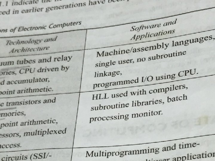
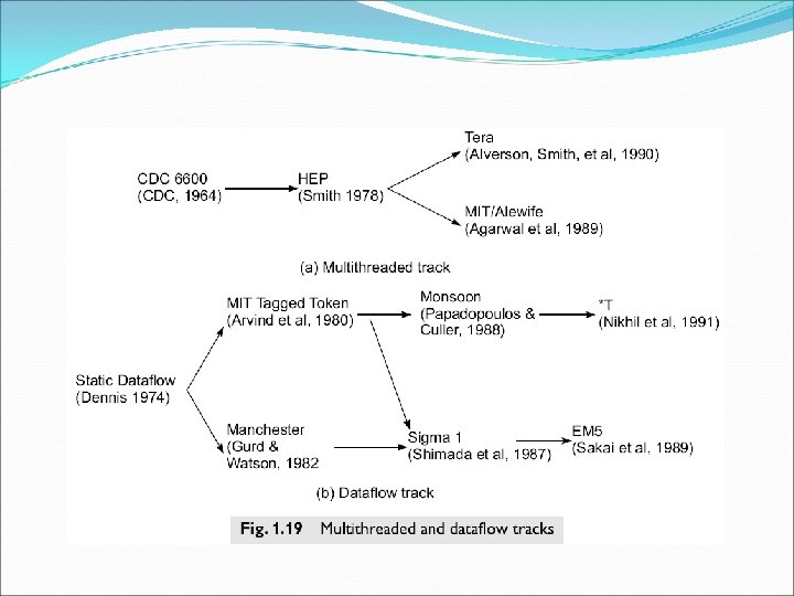
Evolution of Computer Architecture

FLYNN’S CLASSIFICATION

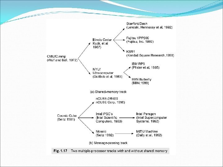
Parallel/Vector computers Execute programs on MIMD mode. 2 major classes: 1. shared-memory multiprocessors 2. message-passing multicomputers.

System attributes to performance Turn around Time : -It is the time which includes disk and memory access, input and output activities, compilation time , OS overhead and CPU time. Clock rate and CPI: processor is driven by a clock with a constant cycle time =t. The inverse of cycle time is the clock rate (f=1/t). The size of the program is determined by its instruction count. (Ic). Different machine instructions may require different number of clock cycles to execute. Therefore CPI (cycles per instruction) becomes an important parameter.

Performance factors Ic= no. of instructions in a given program. Thus the CPU time needed to execute the program is by finding the product of three factors: T= Ic * CPI * t Instruction cycle requires cycle of events: instruction fetch, decode, operand fetch, execution and store results.

In that cycle, only decode and execution phases are carried out in the CPU. The remaining three operations may require access to the memory. Therefore memory cycles is the time needed to complete one memory reference. Therefore CPI is divided into 2 components= processor cycles and memory cycles. Depending on the instruction type, the complete instruction cycle may involve one to as many as four memory references. (one for instruction fetch, two for operand fetch, one for storing result).

Therefore T= Ic * (p + m*k) * t Ic= instruction count P= number of processor cycles. M= number of memory references K= ratio between memory and processor cycle. t= processor cycle time T=CPU Time

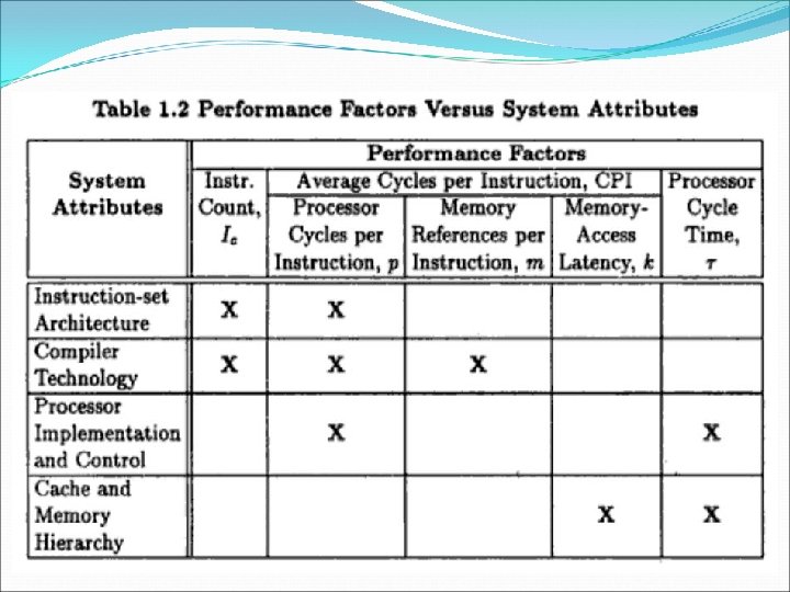
System Attributes The 5 performance factors are influenced by 4 system attributes: Instruction-set architecture Compiler technology CPU implementation and control Cache and memory hierarchy

Instruction-set architecture= Ic, p (processor cycle per instruction) Compiler technology= Ic, p, m (memory references per instruction) CPU implementation and control= p, t (processor cycle time) total processor time needed. Cache and memory hierarchy= affects memory access latency = k, t

MIPS RATE MIPS (millions instructions per second) Throughput rate: how many programs can a system execute per unit time is called system throughput Ws. In multiprogrammed, the system throughput is often lower than the cpu throughput Wp. Because of additional system overheads caused by the i/o, complier and os.

MIPS Let C be the total number of clock cycles needed to execute a program. Therefore CPU time T= C*t= C/F Furthermore CPI= C/Ic T= CPI*Ic*t T= Ic*CPI/f The processor speed measured in MIPS.

mips rate = Ic/T*10^6 = f/CPI*10^6 = f*Ic/ C*10^6 F is clock rate/. Wp= f/Ic*CPI

Implicit and explicit parallelism

Explicit parallelism requires more effort by the programmer to develop a source program using parallel dialects of C, C++, fortron, pascal. Parallelism is specified in the user program. Here the compiler needs to preserve the parallelism.

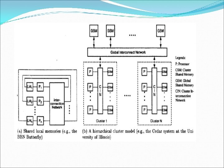
1. 2 Multiprocessors and multicomputers 2 categories of parallel computers 1. 2. 1 - Shared memory multiprocessors 1. 2. 2 - Distributed-memory multicomputers Shared-memory multiprocessors: 3 types: the uniform memory access (UMA) model. The non-uniform memory access (NUMA) The cache-only memory architecture (COMA)

Uniform memory access The physical memory is uniformly shared by all the processors. All processors have equal access time to all memory words. Each processor may use its own private cache. Peripherals are also shared in the same fashion. Multiprocessors are called tightly coupled systems due to high degree of resource sharing. The system interconnect takes the form of a common bus, a crossbar switch or a multistage network.

Uniform memory access

UMA model is suitable for general purpose and timesharing applications. When all processors have equal access time to all the peripheral devices, the system is called a symmetric multiprocessor. In an asymmetric multiprocessor, only one or a subset of processors are executive capable. An executive or a master processors can execute the operating system and handle i/o. the remaining processor have no i/o capabilities, thus are called attached processors.

NUMA model In this the access time varies with the location of the memory word. The shared memory is physically distributed to all processors called local memories. The collection of all local memories forms a global address space accessible by all processors. It is easier to access a local memory with a local processor. The access of remote memory attached to other processors take longer due to added delay through interconnection network.

COMA model The COMA model is a special case of a NUMA machine, in which the distributed main memories are converted to caches. All the caches form a global address space. Remote cache access is assisted by the distributed cache directories.

Distributed memory multicomputers NORMA= no remote memory access. Multicomputer generations: 1 st- 1983 -1987 - based on processor board technology using hypercube architecture and s/w controlled message switching. Eg. Caltech Cosmic and Intel i. PSC/1. 2 nd 1988 -1992 - implemented with mesh connected architecture and a software environment for mediumgrain distributed computing. Eg. Intel paragon and the Parsys Supernode 1000. The 3 rd 1992 -1997 is expected to be fine-grain multicomputers. Eg. MIT-J Machine, Caltech Mosaic

Classification of MIMD computers

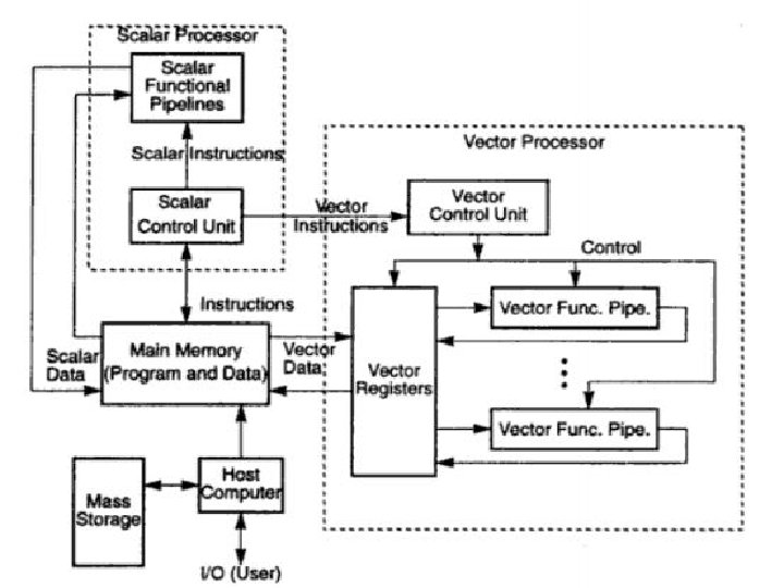
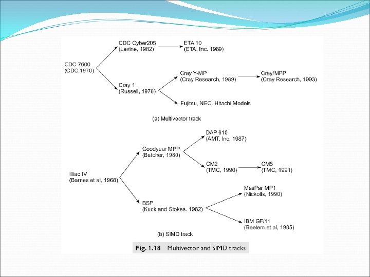
Vector supercomputers A vector supercomputer is built with a scalar processor. Program and data are first loaded into the main memory through a host computer. All instructions are decoded by the scalar control unit. If scalar= goes to scalar processor. If vector= sent to vector control unit.

• The diagram shown is a register to register architecture. • Vector registers are used to hold the vector operands, intermediate and final results. Cray series=fixed length vector registers. • Fujitsu VP 2000= dynamically. • Memory-to-memory= vector operands and results are directly retrieved and stored from the main memory. Eg. 512 bits as in cyber 205.

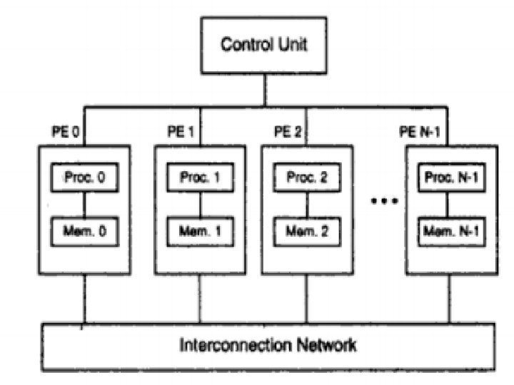
SIMD Supercomputers • An operational model of an SIMD computer is specified by a tuple. • M= {N, C, I, M, R} • N= no. of processing elements. • C= set of instructions directly executed by the control unit. • I= is the set of instructions broadcast by the cu to all pe’s for parallel execution. • M= set of masking scheme, where mask partitions the set of PE’s into enabled and disabled. • R= set of data routing functions, specifying various patterns for inter-pe communications.

PRAM AND VLSI MODELS The ideal models provide a convenient framework for developing parallel algorithms without worry about the implementation details of physical constraints. The models can be used to obtain theoretical performance bounds on parallel computers or to estimate VLSI complexity on chip area and execution time before the chip is fabricated.

Parallel Random Access Machine (PRAM) Time and Space complexity Asymptotic space complexity refers to storage of large problems Non deterministic algorithms

PRAM Models Uni processor computers were modeled as a random access machines By Sheperdson and Sturgis. Parallel random –access machine model has been developed by Fortune and Wyllie. For modeling idealized parallel computers with zero synchronization or memory access overhead. This PRAM model will be used for parallel algorithm development and for scalability and complexity analysis.

PRAM Model An N- Processor PRAM has a globally addressable memory. The shared memory can be distributed among the processors or centralized In one place. These processors work on a synchronized read memory compute and write memory cycles.

4 memory-update options are possible 1. Exclusive read (ER)= this allows only one processor to read from any memory location in one cycle. 2. Exclusive write (EW)= this allows at most one processor to write into memory location. 3. Concurrent read (CR)= multiple processors to read from the same memory location in the same cycle. 4. Concurrent write (CW)= allows simultaneous writes to the same memory. In order to avoid confusion, some policy must be set up to resolve the write conflicts.

Pram variants 1. EREW-PRAM model= this model forbids more than one processor from reading or writing the same memory cell simultaneously. 2. CREW-pram model 3. ER-CW pram model 4. CRCW-PRAM model

Discrepancy with physical models In reality these models don’t exist PRAM operates in synchronized MIMD mode with shared memory. EREW and CRCW are the most popular models. PRAM models will be used for scalability and performance comparison. PRAM Models can put a upper bound and lower bound on the performance of a system.

To resolve concurrent writes 1. common- all writes stores the same value to the memory location. 2. Arbitrary- any one of the values written may remain, the others are ignored. 3. Minimum- minimum value is selected. 4. Priority- the values written are combined using some associative functions such as summation or maximum value.

VLSI Complexity Model