Chapter 1 Data Analysis Section 1 3 Describing

Chapter 1 Data Analysis Section 1. 3 Describing Quantitative Data with Numbers

Displaying Quantitative Data with Numbers LEARNING TARGETS By the end of this section, you should be able to: ü CALCULATE measures of center (mean, median) for a distribution of quantitative data. ü CALCULATE and INTERPRET measures of variability (range, standard deviation, IQR) for a distribution of quantitative data. ü EXPLAIN how outliers and skewness affect measures of center and variability. ü IDENTIFY outliers using the 1. 5 × IQR rule. ü MAKE and INTERPRET boxplots of quantitative data. ü Use boxplots and numerical summaries to COMPARE distributions of quantitative data. Starnes/Tabor, The Practice of Statistics

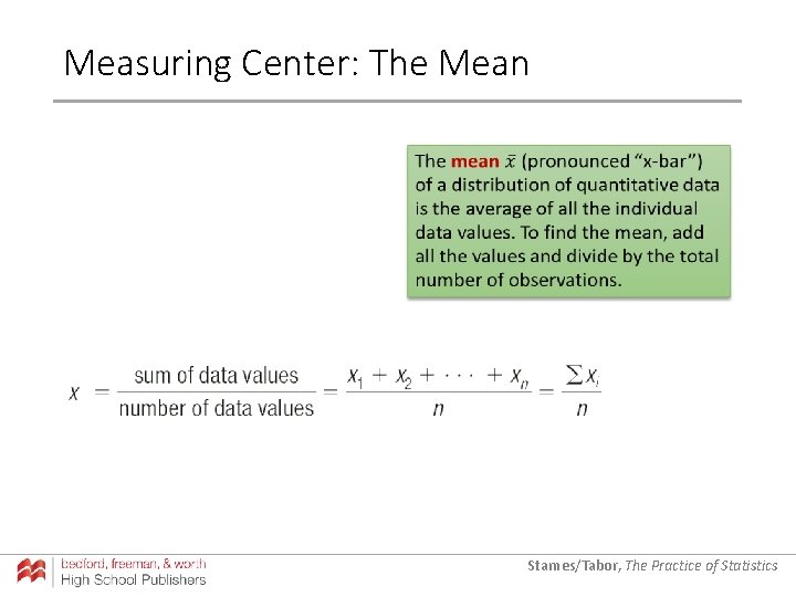
Measuring Center: The Mean Starnes/Tabor, The Practice of Statistics

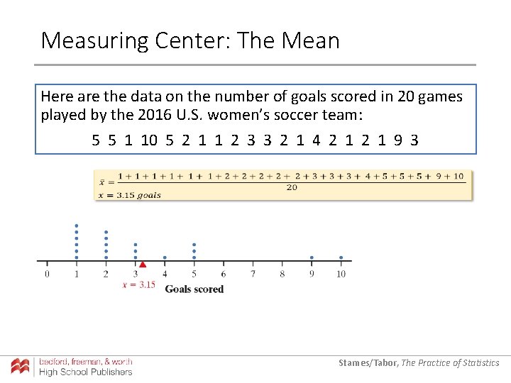
Measuring Center: The Mean Here are the data on the number of goals scored in 20 games played by the 2016 U. S. women’s soccer team: 5 5 1 10 5 2 1 1 2 3 3 2 1 4 2 1 9 3 Starnes/Tabor, The Practice of Statistics

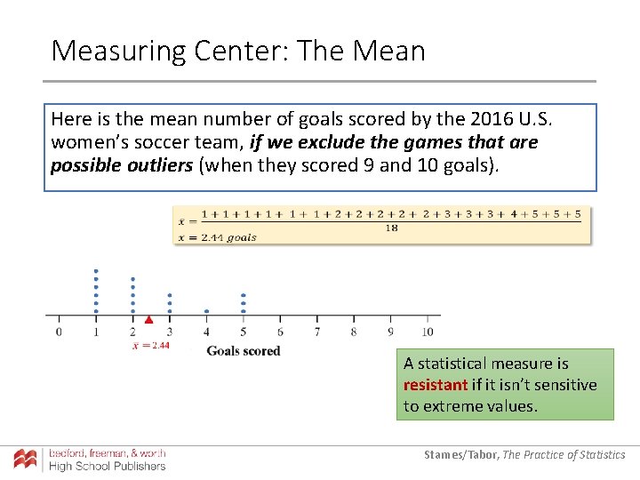
Measuring Center: The Mean Here is the mean number of goals scored by the 2016 U. S. women’s soccer team, if we exclude the games that are possible outliers (when they scored 9 and 10 goals). A statistical measure is resistant if it isn’t sensitive to extreme values. Starnes/Tabor, The Practice of Statistics

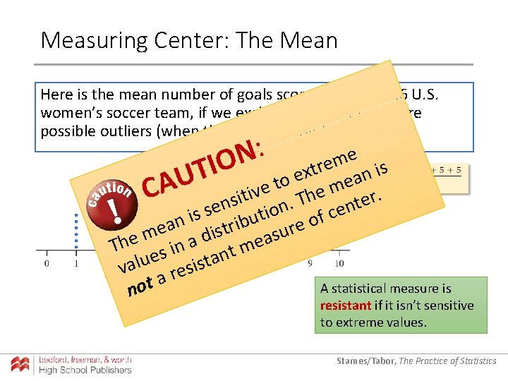
Measuring Center: The Mean Here is the mean number of goals scored by the 2016 U. S. women’s soccer team, if we exclude the games that are possible outliers (when they scored 9 and 10 goals). : N IO e m e tr an is x T e U o e t m A e iv. The C. t r i s e t n n se ution e c s i f o n b i a e r st u i m s d a e Th n m i t s n e a u t s i s val e r a t A statistical measure is no resistant if it isn’t sensitive to extreme values. Starnes/Tabor, The Practice of Statistics

Measuring Center: The Median The median is the midpoint of a distribution, the number such that about half the observations are smaller and about half are larger. To find the median, arrange the data values from smallest to largest. • If the number n of data values is odd, the median is the middle value in the ordered list. • If the number n of data values is even, the median is the average of the two middle values in the ordered list. Starnes/Tabor, The Practice of Statistics

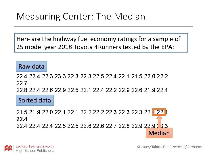
Measuring Center: The Median Here are the highway fuel economy ratings for a sample of 25 model year 2018 Toyota 4 Runners tested by the EPA: Raw data 22. 4 22. 3 23. 3 22. 5 22. 4 22. 1 21. 5 22. 0 22. 2 22. 7 22. 8 22. 4 22. 6 22. 9 22. 5 22. 1 22. 4 22. 2 22. 9 22. 6 21. 9 22. 4 Sorted data 21. 5 21. 9 22. 0 22. 1 22. 2 22. 3 22. 4 22. 5 22. 6 22. 7 22. 8 22. 9 23. 3 Median Starnes/Tabor, The Practice of Statistics

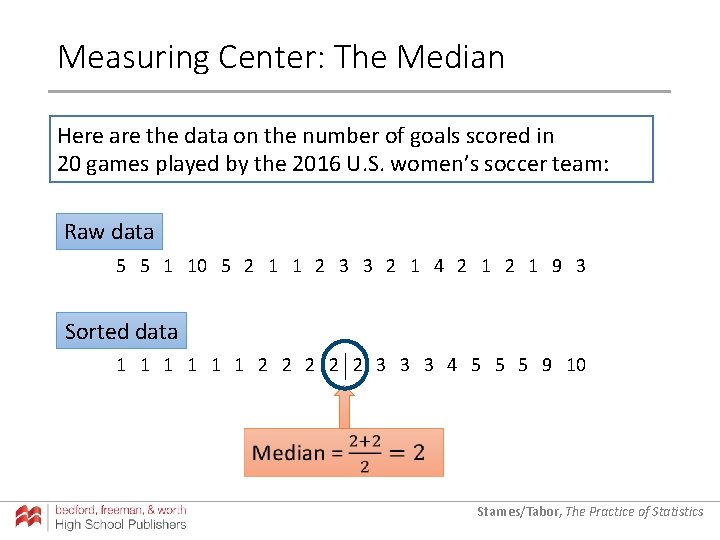
Measuring Center: The Median Here are the data on the number of goals scored in 20 games played by the 2016 U. S. women’s soccer team: Raw data 5 5 1 10 5 2 1 1 2 3 3 2 1 4 2 1 9 3 Sorted data 1 1 1 2 2 2 3 3 3 4 5 5 5 9 10 Starnes/Tabor, The Practice of Statistics

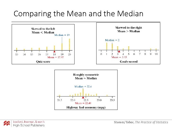
Comparing the Mean and the Median Starnes/Tabor, The Practice of Statistics

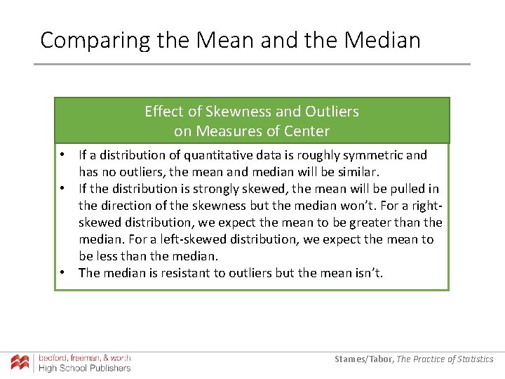
Comparing the Mean and the Median Effect of Skewness and Outliers on Measures of Center • If a distribution of quantitative data is roughly symmetric and has no outliers, the mean and median will be similar. • If the distribution is strongly skewed, the mean will be pulled in the direction of the skewness but the median won’t. For a rightskewed distribution, we expect the mean to be greater than the median. For a left-skewed distribution, we expect the mean to be less than the median. • The median is resistant to outliers but the mean isn’t. Starnes/Tabor, The Practice of Statistics

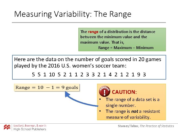
Measuring Variability: The Range The range of a distribution is the distance between the minimum value and the maximum value. That is, Range = Maximum – Minimum Here are the data on the number of goals scored in 20 games played by the 2016 U. S. women’s soccer team: 5 5 1 10 5 2 1 1 2 3 3 2 1 4 2 1 9 3 CAUTION: • The range of a data set is a single number. • The range is not a resistant measure of variability. Starnes/Tabor, The Practice of Statistics

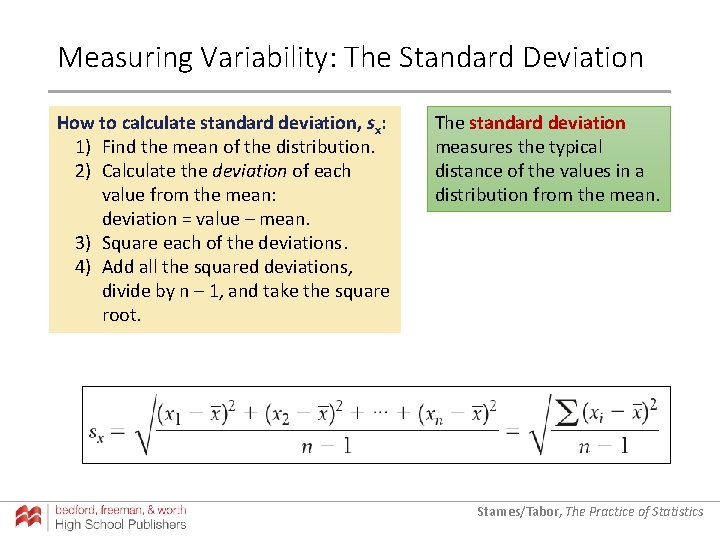
Measuring Variability: The Standard Deviation How to calculate standard deviation, sx: 1) Find the mean of the distribution. 2) Calculate the deviation of each value from the mean: deviation = value – mean. 3) Square each of the deviations. 4) Add all the squared deviations, divide by n – 1, and take the square root. The standard deviation measures the typical distance of the values in a distribution from the mean. Starnes/Tabor, The Practice of Statistics

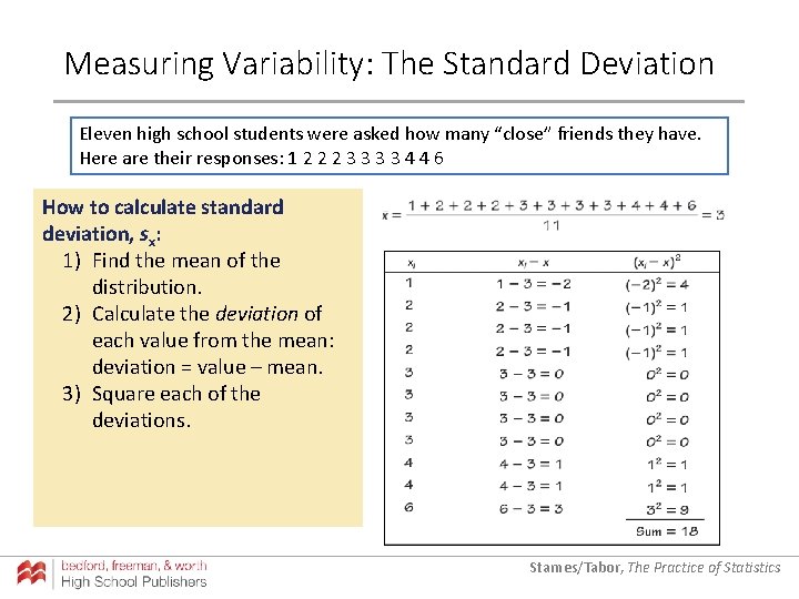
Measuring Variability: The Standard Deviation Eleven high school students were asked how many “close” friends they have. Here are their responses: 1 2 2 2 3 3 4 4 6 How to calculate standard deviation, sx: 1) Find the mean of the distribution. 2) Calculate the deviation of each value from the mean: deviation = value – mean. 3) Square each of the deviations. Starnes/Tabor, The Practice of Statistics

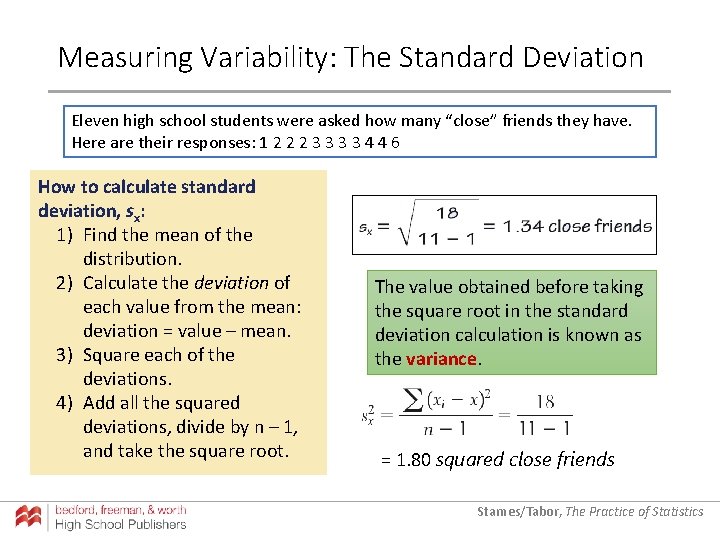
Measuring Variability: The Standard Deviation Eleven high school students were asked how many “close” friends they have. Here are their responses: 1 2 2 2 3 3 4 4 6 How to calculate standard deviation, sx: 1) Find the mean of the distribution. 2) Calculate the deviation of each value from the mean: deviation = value – mean. 3) Square each of the deviations. 4) Add all the squared deviations, divide by n – 1, and take the square root. The value obtained before taking the square root in the standard deviation calculation is known as the variance. = 1. 80 squared close friends Starnes/Tabor, The Practice of Statistics

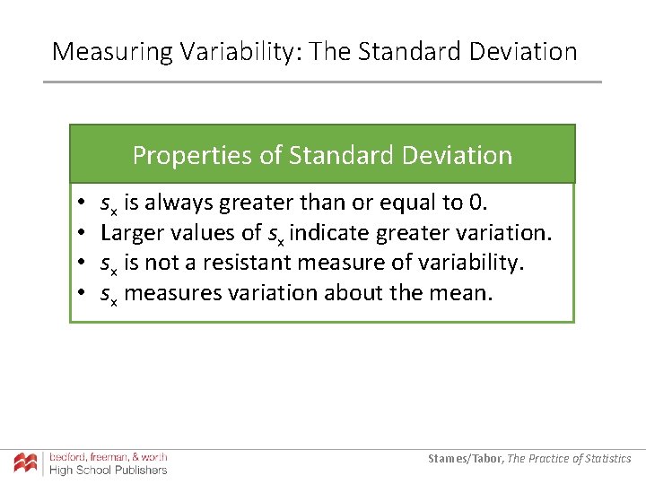
Measuring Variability: The Standard Deviation Properties of Standard Deviation • • sx is always greater than or equal to 0. Larger values of sx indicate greater variation. sx is not a resistant measure of variability. sx measures variation about the mean. Starnes/Tabor, The Practice of Statistics

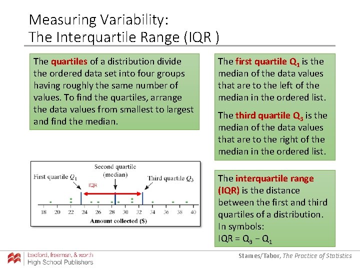
Measuring Variability: The Interquartile Range (IQR ) The quartiles of a distribution divide the ordered data set into four groups having roughly the same number of values. To find the quartiles, arrange the data values from smallest to largest and find the median. The first quartile Q 1 is the median of the data values that are to the left of the median in the ordered list. The third quartile Q 3 is the median of the data values that are to the right of the median in the ordered list. The interquartile range (IQR) is the distance between the first and third quartiles of a distribution. In symbols: IQR = Q 3 − Q 1 Starnes/Tabor, The Practice of Statistics

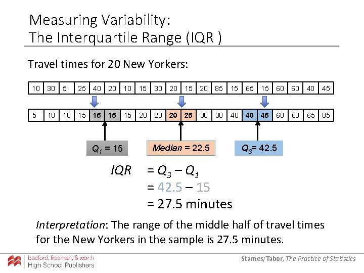
Measuring Variability: The Interquartile Range (IQR ) Travel times for 20 New Yorkers: 10 30 5 25 40 20 10 15 30 20 15 20 85 15 60 60 40 45 5 10 10 15 15 20 20 20 25 30 30 40 40 45 60 60 65 85 Q 1 = 15 IQR Median = 22. 5 Q 3= 42. 5 = Q 3 – Q 1 = 42. 5 – 15 = 27. 5 minutes Interpretation: The range of the middle half of travel times for the New Yorkers in the sample is 27. 5 minutes. Starnes/Tabor, The Practice of Statistics

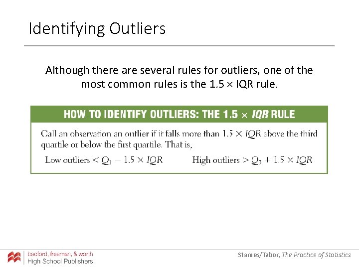
Identifying Outliers Although there are several rules for outliers, one of the most common rules is the 1. 5 × IQR rule. Starnes/Tabor, The Practice of Statistics

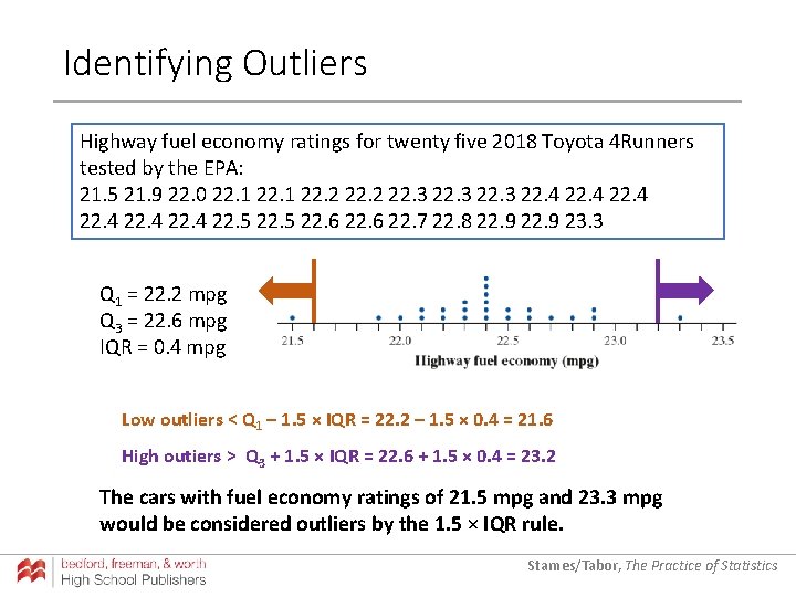
Identifying Outliers Highway fuel economy ratings for twenty five 2018 Toyota 4 Runners tested by the EPA: 21. 5 21. 9 22. 0 22. 1 22. 2 22. 3 22. 4 22. 5 22. 6 22. 7 22. 8 22. 9 23. 3 Q 1 = 22. 2 mpg Q 3 = 22. 6 mpg IQR = 0. 4 mpg Low outliers < Q 1 – 1. 5 × IQR = 22. 2 – 1. 5 × 0. 4 = 21. 6 High outiers > Q 3 + 1. 5 × IQR = 22. 6 + 1. 5 × 0. 4 = 23. 2 The cars with fuel economy ratings of 21. 5 mpg and 23. 3 mpg would be considered outliers by the 1. 5 × IQR rule. Starnes/Tabor, The Practice of Statistics

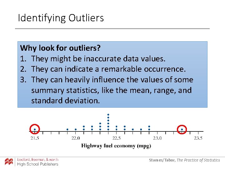
Identifying Outliers Why look for outliers? 1. They might be inaccurate data values. 2. They can indicate a remarkable occurrence. 3. They can heavily influence the values of some summary statistics, like the mean, range, and standard deviation. Starnes/Tabor, The Practice of Statistics

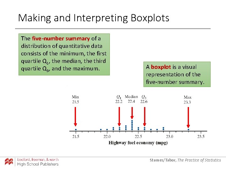
Making and Interpreting Boxplots The five-number summary of a distribution of quantitative data consists of the minimum, the first quartile Q 1, the median, the third quartile Q 3, and the maximum. A boxplot is a visual representation of the five-number summary. Starnes/Tabor, The Practice of Statistics

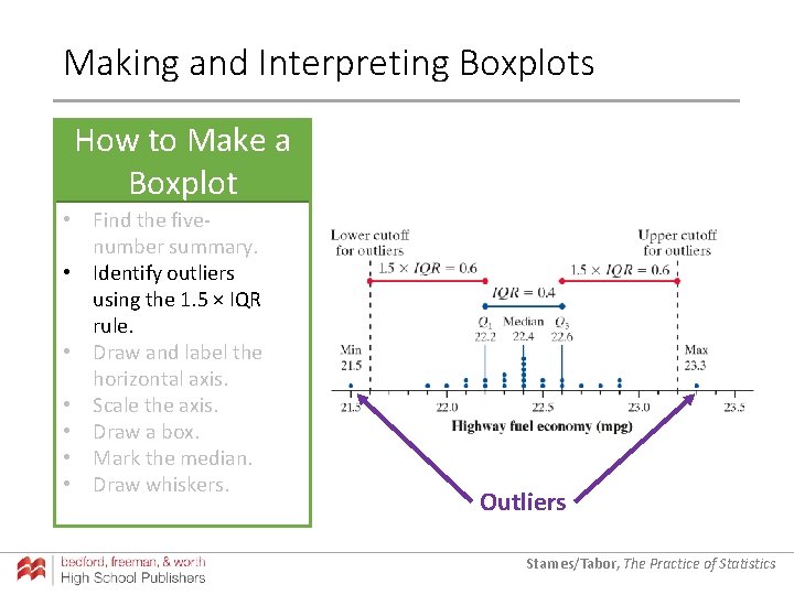
Making and Interpreting Boxplots How to Make a Boxplot • Find the fivenumber summary. • Identify outliers using the 1. 5 × IQR rule. • Draw and label the horizontal axis. • Scale the axis. • Draw a box. • Mark the median. • Draw whiskers. Outliers Starnes/Tabor, The Practice of Statistics

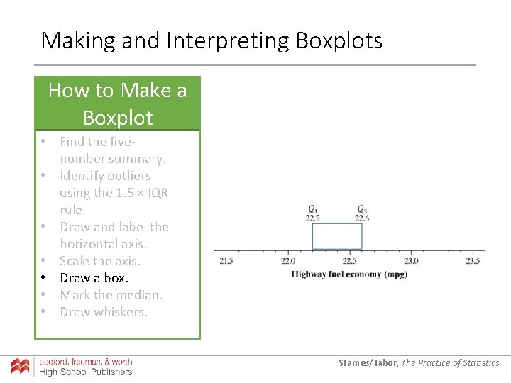
Making and Interpreting Boxplots How to Make a Boxplot • Find the fivenumber summary. • Identify outliers using the 1. 5 × IQR rule. • Draw and label the horizontal axis. • Scale the axis. • Draw a box. • Mark the median. • Draw whiskers. Starnes/Tabor, The Practice of Statistics

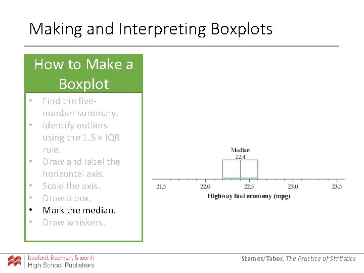
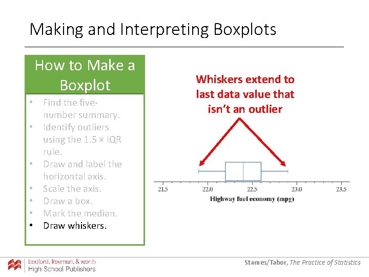
Making and Interpreting Boxplots How to Make a Boxplot • Find the fivenumber summary. • Identify outliers using the 1. 5 × IQR rule. • Draw and label the horizontal axis. • Scale the axis. • Draw a box. • Mark the median. • Draw whiskers. Whiskers extend to last data value that isn’t an outlier Starnes/Tabor, The Practice of Statistics

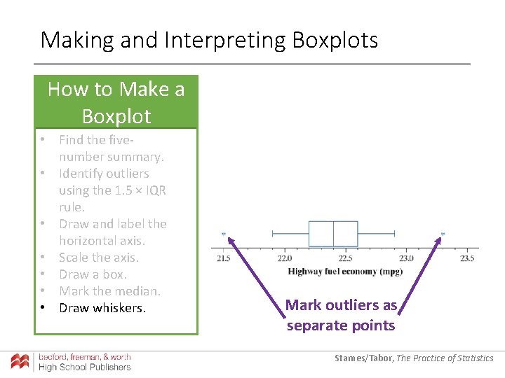
Making and Interpreting Boxplots How to Make a Boxplot • Find the fivenumber summary. • Identify outliers using the 1. 5 × IQR rule. • Draw and label the horizontal axis. • Scale the axis. • Draw a box. • Mark the median. • Draw whiskers. Mark outliers as separate points Starnes/Tabor, The Practice of Statistics

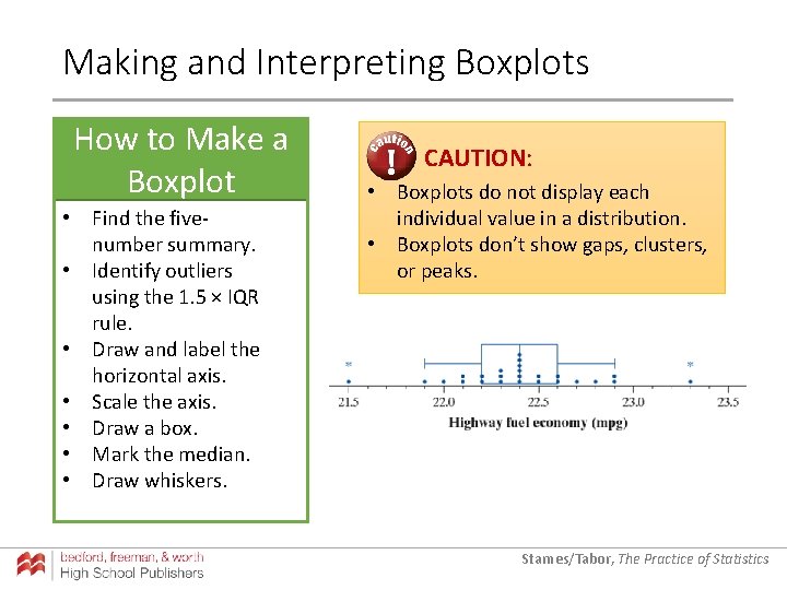
Making and Interpreting Boxplots How to Make a Boxplot • Find the fivenumber summary. • Identify outliers using the 1. 5 × IQR rule. • Draw and label the horizontal axis. • Scale the axis. • Draw a box. • Mark the median. • Draw whiskers. CAUTION: • Boxplots do not display each individual value in a distribution. • Boxplots don’t show gaps, clusters, or peaks. Starnes/Tabor, The Practice of Statistics

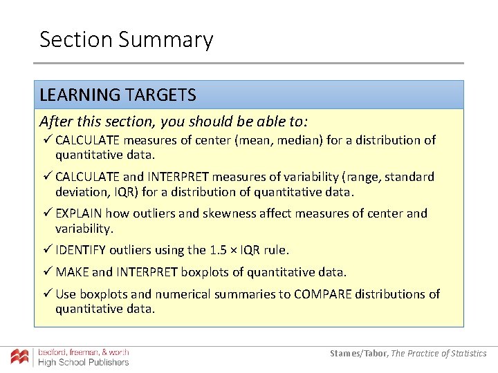
Section Summary LEARNING TARGETS After this section, you should be able to: ü CALCULATE measures of center (mean, median) for a distribution of quantitative data. ü CALCULATE and INTERPRET measures of variability (range, standard deviation, IQR) for a distribution of quantitative data. ü EXPLAIN how outliers and skewness affect measures of center and variability. ü IDENTIFY outliers using the 1. 5 × IQR rule. ü MAKE and INTERPRET boxplots of quantitative data. ü Use boxplots and numerical summaries to COMPARE distributions of quantitative data. Starnes/Tabor, The Practice of Statistics