Chapter 1 Consumption Saving and Investment PierreRichard Agnor

Chapter 1 Consumption, Saving and Investment © Pierre-Richard Agénor The World Bank

l l Consumption and Saving Investment

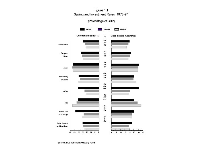
l l l Basic facts (Figure 1. 1): Gross domestic saving rates in developing countries are higher than the rates in industrial countries (highest in Asia). Investment rate follows similar pattern (highest in Asia). Foreign saving is particularly large in Sub-Saharan Africa.

Consumption and Saving l l Keynesian Approach Permanent Income Hypothesis The Life-Cycle Model è The Basic Framework è Age and Dependency Ratio Other Determinants è Income Levels and Income Uncertainty è Intergenerational Links è Liquidity Constraints è Inflation and Macroeconomic Stability è Government Saving

The Debt Burden and Taxation è Social Security, Pensions and Insurance è Changes in the Terms of Trade è Financial Deepening è Household and Corporate Saving Empirical Evidence è l

Keynesian Approach l Consumption is a function of disposable income: C = (1 - s)(Y - T), l l C current consumption, Y - T disposable income; 0 < s < 1 marginal propensity to save. Merits: First approximation in empirical macroeconomic models. A reflection of the behavior of consumers subject to liquidity constraints.

The Permanent Income Hypothesis l l l Consumption is a function of permanent income. Example : Consumers are identical and live for only two periods, 1 and 2. Assume perfect foresight. Budget constraint for period 1: A 1 - A 0 = Y 1 - T 1 + r. A 0 - C 1 (1) A: stock of financial assets, Y - T disposable income; r: real interest rate (constant).

l Budget constraint for period 2, in the absence of bequest: C 2 = Y 2 - T 2 + (1+r)A 1 l l (2) Eliminate A 1 from (1) by using (2). Yield the household’s intertemporal budget constraint: C 2 Y 2 - T 2 C 1 + ––––– = (1+r)A 0 + (Y 1 - T 1) + –––– 1+r (3)

l l Simple version of the model: Household’s objective is to maintain a perfectly stable (or smooth) consumption path, C 1 = C 2. Divide its lifetime resources equally among each period of life. Amount consumed by the household in each period is equal to its permanent income, Yp. Yp : level of income that gives the household the same present value of its lifetime resources as that implied by its intertemporal budget constraint.

Using equation (3) intertemporal budget constraint is l Yp Y 2 - T 2 Yp + ––––– = (1+r)A 0 + (Y 1 - T 1) + –––– 1+r l Then Yp becomes: 1+r Y 2 - T 2 Yp = (–––––){(1+r)A 0 + (Y 1 - T 1) + ––––––– } 2+r 1+r

l If A 0 = 0 and r = 0, YP becomes an exact average of present and future disposable income. (Y 1 - T 1 )+ (Y 2 - T 2 ) Yp = ––––––––––– 2 Implications: l Saving (in period 1) is the difference between disposable income and permanent income. S 1 = Y 1 - C 1 = Y 1 - Y p

l Transitory income : YT = Y 1 - Yp l This forms the basis for a number of empirical tests.

The Life-Cycle Model l l Importance of variations in the structure of income during life cycle. Figure 1. 2: stylized pattern of income, consumption, and savings predicted by the standard life-cycle model.

Basic Framework: l l Two period framework. Life time budget constraint : C 2 C 1 + ––––– = W 1 1+r W 1: life-time wealth. (4)

l Suppose that the household’s preferences are intertemporally additive : u(C 2) U = u(C 1) + –––––– 1+ (5) U: life-time utility; : rate of time preference which measures the degree of impatience.

l l Maximization of (5) with respect to C 1 and C 2 subject to the life-time budget constraint (4). By forming the Lagrangien expression: C 2 L = U + [C 1 + ––––– - W 1] 1+r l : Lagrange multiplier. The first order optimality conditions are given by: u’(C 1 ) = , u’(C 2) = –––––. 1+ 1+r –––––––

Combining these two equations obtain Euler equation : l 1+r u’(C 1 ) = –––––u’(C 2) 1+ l l When = r, we obtain C 1 = C 2. The model becomes the simple version of permanent income hypothesis. Assume constant elasticity of substitution : - - -1/ U = {C 1 + C 2 /(1+ )} where > 1.

l The elasticity of substitution between period 1 and period 2 consumption, , is : = 1/(1+ ). l Euler equation becomes : -1/ C 1 l 1+r -1/ = (–––––)C 2 1+ Taking logarithms of both side 1+r ln(C 2/C 1) = ln(––––---) (r - ) 1+

l l l measures the responsiveness of the change in consumption between the two periods to changes in interest rate, r. The effect of the change in r on consumption and saving (in period 1) is indeterminate. Conflict between income and substitution effects. The greater is , the greater will be the reduction in C 1 (relative to C 2) induced by a rise in r. If is sufficiently large: effect of substitution dominates; an increase in r reduces consumption and raises saving.

Age and Dependency Ratio l l l Predictions of life-cycle model The young will save relatively little as they anticipate increases in their future income. Middle-aged individuals, who are nearing the peak of their earnings, tend to save the most, in anticipation of relatively low incomes after retirement. The elderly tend to have a low, or even negative, saving rate, although the desire to leave a bequest or to cover the contingency of living longer than expected could provide motivation for saving even after retirement.

l Implication: Aggregate saving rate will tend to fall in response to dependency ratio, measured as è youth dependency ratio (ratio of under-20 age group to the 20 -64 age group); ratio of the elderly to the working age population. Distribution of assets among the population affects the consumption and saving patterns at the aggregate level. The larger the share of total wealth held by the middle-aged households, the higher the saving rate, and the higher the growth rate of income in a given country. è l l

l Remark : demographic factors such as the share of the working population relative to the that of retired persons are likely to explain only the long-term trends in saving.

Other Determinants

Income levels and income uncertainty l l Recent empirical research has highlighted the fact that at low or subsistence levels of income, the saving rate is also low. Two implications: è in low-income countries the response of saving to changes in real interest rate is likely to be weak; è changes in income distribution can have important effects on measured saving rates at the aggregate level.

l l Increased uncertainty regarding future income will enhance the precautionary motive for saving. Sources of income uncertainty : Many households in developing countries derive their incomes from agriculture. In that sector, incomes can be subject to relatively large fluctuations resulting from variations in climatic conditions or changes in domestic and the world prices of agricultural commodities. Macroeconomic instability.

Intergenerational Links l l Intergenerational links are likely to be strong in developing countries (role of extended family). These links can affect consumption and saving in two ways: è lengthen the effective planning horizon over which households make their consumption and saving decisions; è affect household preferences (by affecting, for example, the degree to which the marginal utility of consumption).

Liquidity Constraints l l l Consumption smoothing requires well-functioning financial markets to allow agents to borrow and lend across periods. In many developing countries, well-developed financial markets either do not exist, or not function very well. Households often have limited access to credit markets, and credit rationing may be pervasive.

l l Liquidity constraints affect the ability of households to transfer resources across time periods as well as across uncertain states of nature relative to income. Consequence : consumption tends to be highly correlated with current income, rather than permanent income or life-cycle wealth. In the presence of liquidity constraints, financial liberalization can have an adverse effect on saving rates. Increased access to these markets will allow individuals to bring forward their consumption (reduce saving).

Inflation and Macroeconomic Stability l l l If households are net creditors, an increase in the inflation rate may lower real value of wealth. To offset this, they raise their saving rate. The variability of inflation (measure of macroeconomic stability) may affect saving by increasing uncertainty about future income. Precautionary motive : a high degree of price variability may lead to an increase in the saving rate.

Government Saving l l l Key feature of the life-cycle model: saving behavior is directly influenced by households’ assessments of their future disposable income. Key variable that affects these assessments is government policy, particularly government saving or dissaving. Three major interpretations of the relationship between government and private saving:

l l Conventional view: Assume a fall in government saving (resulting from a tax cut or a bond-financed increase in government spending). This will tend to raise consumption and reduce saving by myopic households (that is, households who care solely about the present). Reason: they shift the tax burden from present to future generations. Decline in government saving will lead to a decline in national saving.

l l The Keynesian view Higher temporary government dissaving. Consumption and income increase in the presence of under-utilized production capacity: multiplier effect. Higher income will raise private saving. Whether or not this increase in private saving is large enough to offset the initial decline in government saving is a priori ambiguous.

l l l The Ricardian equivalence view Predicts that a rise in the budget deficit resulting from a tax cut will have no effect on the national saving rate because private saving will rise by an equivalent amount in anticipation of future tax liabilities. If individuals are rational and far-sighted, they will realize that a permanent rise in government spending today must be paid for either now or later. They will increase saving by an equivalent amount.

l Critics for the assumptions of Ricardian equivalence from the analytical point of view: è consumers are far-sighted; è successive generations are linked by altruistically motivated bequests; è consumers do not face liquidity constraints; è taxes are nondistortionary.

l l Empirical results for developing countries is against Ricardian equivalence. Reason: although individuals may form expectations about their future tax liabilities in a systematic way, liquidity constraint may prevent them from acting on these expectations.

Social Security, Pensions, and Insurance l l The availability of formal public pension and social security schemes may cause to lower the private saving rate. Channels implied by the life-cycle model: è by redistributing income to the elderly; è by reducing the need to save for retirement (if there is no reduction of the retirement age); è by curbing the need for precautionary saving to cover the contingency of living longer than expected.

l l The impact of increased social security benefits on national saving depend on the effect that such changes on public saving. Private pension plans have been developed in many developing countries in recent years. In principle, individuals should view their contributions to funded private pensions as a perfect substitute for other forms of saving. But, in practice, individuals do not seem to fully take into account their pension contributions in determining their saving behavior.

l l l Result : introduction of private pension plans is often accompanied by an increase in national saving rates. Conclusion of Holzmann (1997) in the case of Chile. Availability of various kinds of insurance: è health insurance ; è unemployment insurance ; è personal loss and liability insurance. They influence saving behavior. To the extent that insurance plans limit expected outlays for contingencies and emergencies, they tend to reduce income uncertainty and therefore the need for precautionary saving.

Changes in the Terms of Trade l l Movements in terms-of-trade has an important effect on saving. Harberger-Laursen-Meltzer Effect: predicts a positive relationship between changes in the termsof-trade and saving, through their positive effect on wealth and income. Predictions: Temporary decrease in terms of trade leads to decrease in current income compared to future income thus leads to a decrease in saving. If permanent deterioration in the terms of trade leads to reduction in both permanent and transitory income, no effect on saving.

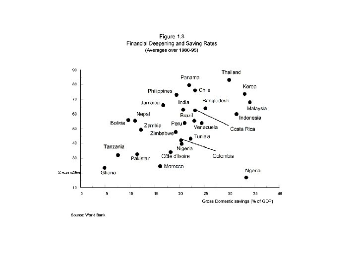
Financial Deepening l l Financial development may affect saving both directly and indirectly: è reduction in cost of intermediation leads to increase in the return to saving; è increased efficiency in the process of financial intermediation leads to an expansion of investment and stimulates the rate of economic growth; è increase in income leads to an increase in saving. Figure 1. 3: positive relationship between gross domestic saving rates and an indicator of financial deepening.

Household and Corporate Saving l l Forgoing discussion focused only on saving by households. This focus justified in the many developing countries where private saving rates are essentially determined by household behavior. However corporate saving (retained earnings) may also be significant. They may respond to different variables than those affecting the decisions of households.

l l l Importance of this distinction in the aggregate private saving depends on households’ responses to higher corporate saving. If firms retain more earnings, households may have less by a corresponding amount: è In such conditions, households pierce the corporate veil. è Aggregate private saving behavior will largely reflect household behavior. Example: Colombia (Figure 1. 4).

Empirical Evidence l l Masson, Bayoumi, and Samiei (1995) Edwards (1996 c) Dayal-Gulati and Thimann (1997) Loayza, Schmidt-Hebbel and Servén (1999).

Masson, Bayoumi, and Samiei (1995) l l Used cross-country database (developing countries) to study determinants of private saving. Results: increase in public saving associated with higher national saving, suggesting Ricardian equivalence does not hold; decrease in age dependency ratio raises private saving; increase in per capita income raises private saving;

l l l changes in real interest rate had no significant effect on saving; increases in foreign saving increases both investment and consumption; terms-of-trade windfalls have a positive but transitory effect on saving.

Edwards (1996 c) l l Used both developing and industrialized countries. Significant determinants of private saving rate: è rate of growth of per capita income; è monetization ratio (indicator of financial deepening); è foreign saving (negative effect); è government saving (negative effect); è social securities (negative effect).

Dayal-Gulati and Thimann (1997) l l Used both Southeast Asia and Latin America countries. Determinants of private saving rate: è terms of trade shock: positive effect; è government saving: partially crowd out private saving; è social security expenditures: negative effect; è fully funded pension schemes: positive effect; è macroeconomic stability: positive effect; è financial deepening: positive effect; è per capita income: positive effect.

Loayza et al. (1999) l l Used an extensive cross-country database to study determinants of private saving. A novelty of the analysis : distinction between short - and long-term determinants of saving rate. This distinction is highly significant in their empirical results. Main findings: Macroeconomic uncertainty (the variance of inflation) had a positive effect on private saving rates. Consistent with the precautionary motive.

l l l Public sector saving had a negative but less than proportional effect on private saving. Ricardian equivalence does not hold in strict terms. Real interest rates had no significant effect on saving. Terms-of-trade improvements were positively associated with private and national saving rates. Limitations: Effect of interest rates on saving may be nonlinear. Asymmetric effects of terms-of-trade.

Investment l l l The Flexible Accelerator The Cost of Capital Uncertainty and Irreversibility Other Determinants of Investment è Credit Rationing è Foreign Exchange Constraint è The Real Exchange Rate è Public Investment è Macroeconomic Stability è The Debt Burden Effect Empirical Evidence

Flexible Accelerator l Assumption: production technology is characterized by a fixed relationship between the desired capital stock and the level of output. ~ K = ya, > 0, ~ l K: desired capital stock; ya: expected output. Suppose actual capital adjustment is: ~ K = (K - K-1), 0 < < 1.

l Gross private investment: Ip = K + K-1, 0 < < 1, : depreciation rate l When = 0, = 1, and expected future output is approximated by current output: Ip = y. l l It relates investment linearly to changes in current output. Limitation: profitability, uncertainty, and the cost of capital play no role.

Cost of Capital l l View investment as depending inversely on the user cost of capital. Three components of user cost of capital: opportunity cost; measured by the interest rate the firm would receive if it sold the capital and invested the proceeds; cost resulting from the depreciation of the capital good; capital loss (or gain) resulting from the fact that the price of capital may be falling (rising).

l Cost of capital: c. K = PK [i + - ( PK / PK)], l i: interest rate; PK the price of one unit of capital; : depreciation rate; i - PK /PK : real interest rate measured in PK. When combined with the flexible accelerator: ~ K l = ya / c. K Investment is inversely related to the cost of capital services.

l Limitation: it does not account for the impact of uncertainty on the decision to invest.

Uncertainty and Irreversibility l l l Under uncertainty, private investment decisions may be significantly affected by irreversibility effect (essentially due to sunk cost). Because of irreversibility of investment, waiting has value as it gives firms the opportunity to process new information before the decision to invest is taken. Servén (1997) model: Examine the effects of uncertainty and irreversibility on investment.

l l l Assumptions: Risk-neutral firm must decide whether to invest in a project in which the initial cost is completely sunk at the purchase cost PK at the beginning of period t 0 = 0. It yields a return of R 0 at the end of that period. Future demand for the good generated by the project is uncertain; as a result, the rate of return on the project in period t = 1 and beyond, denoted R, is also uncertain.

l Net present value of the anticipated return stream of cash flows associated with the project: R 0 V 0 - PK + + 1+i 1 1+i 2 (1+ )-h. E 0 R, h=0 i: Discount rate, taken to be equal to the rate of return on an alternative investment, such as riskless government bonds. E 0 R: Given the information available at period 0, the expected value of the future return.

l This can be rewritten as: R 0+ E 0 R /i V 0 - PK + 1+i l The conventional net present value criterion suggests that the investment is profitable and thus should be made as long as V 0 > 0. After rearranging terms yields: E 0 R - i. PK R 0 - i. PK + i >0, (33) i. PK: user cost of capital in the case where the depreciation rate is zero.

l With full reversibility of investment, the future would not matter; the optimal decision rule would thus be to invest today as long as: R 0 - i. PK > 0, l (34) i. e. as long as the current return exceeds the user cost of capital. The presence of irreversibility requires taking into account both the difference between the expected return and the user cost of capital (Equation (33)).

l l l But although Equation (33) must hold in an ex ante sense, it may not ex post; the reason is that there is a nonzero probability that at some period t in the future, the inequality Equation (34) may be reversed, that is, R - PK < 0. The firm may thus be locked in an unprofitable investment. There is, therefore, an incentive to delay investment in order to learn more about the factors affecting future return (in the present case, about the state of market demand for the good produced by the firm).

l l To determine how uncertainty affects the decision rule (33), consider first the case where the firm knows for sure that uncertainty will completely vanish in period t = 1 and that the project's returns for t = 2, . . . will remain constant at the level realized in the first period. Suppose then that the firm decides not to invest at all today and to invest next period if and only if the realized return exceeds the user cost of capital.

l In that case, the net present value of the anticipated stream of cash flows: V 1 Pr(R > i PK) { - PK + 1+i 1 1+i 2 (1+i)-h. E 0(R | R > i PK) h=0 Pr(R > i. PK) : probability that the project's return exceeds the cost of capital; E 0(R | R > i. PK): expected value of R, conditional on the project's return exceeding the cost of capital. }

l Comparing V 0 with V 1, the firm is better off investing today if : V 1 - V 0 < 0, (35) E 0(i PK - R | R i PK) R 0 - i PK > Pr(R i PK) i a condition can be written as R 0 - i PK: cost of waiting, given by the net return foregone in period 0 by not investing. (R i PK): value of waiting, given by the irreversible mistake that would be revealed tomorrow if future returns fall short of the user cost of capital.

l The expected present value of such mistake is measured by the right-hand side of Equation (35): è mistake is made with probability Pr(R i PK); è its expected per-period size, given today's information, is E 0(i PK - R | R i PK); è because it accrues every period into the indefinite future, it has to be multiplied by 1/i to transform it to present value terms.

l l l Thus, condition (33) indicates that it is profitable to invest immediately only if the first-period return exceeds the conventionally measured user cost of capital by a margin that is large enough to compensate for the possibility of an irreversible mistake. In other words: if the cost of waiting outweighs the value of waiting. Implication of Equation (35): possibility that in the future R may exceed i. PK has no effect on the investment threshold and thus no effect on the decision to invest today.

l l Reason for this asymmetry: option to wait has no value in those good states of nature in which investing would have been the right decision anyway. Option value of waiting: = max(V 1 -V 0 , 0). l l If V 1 - V 0 < 0, the option has no value, and the optimal decision is to invest today (at period 0). In general, however, the option value of waiting can be large, especially in a highly uncertain environment.

l l As a consequence, uncertainty can become a powerful deterrent to investment even under risk neutrality. Uncertainty may result from various domestic and external sources, including a high degree of volatility in aggregate demand, large movements in the terms of trade and relative prices, and incomplete credibility of adjustment policies. Increased macroeconomic volatility raises the likelihood of bad outcomes (i. e. R i. PK). Result: increase in the spread of the distribution of future returns.

l l l This will raise the critical threshold that the marginal productivity of capital must reach, and thus tend to depress investment. But this does not always hold. If R 0 is uncertain and the investment is partly reversible, then higher uncertainty could hasten investment, by making extreme favorable realizations of R 0 more likely. Reason: firm can avoid the impact of negative outcomes on profitability by shutting down the project (Bar-Ilan and Strange, 1996). Although both the value and the cost of waiting rise with higher uncertainty, the latter rises by a greater amount.

l l The higher the degree of irreversibility (that is, the higher the degree of asymmetry in investment adjustment costs), the more likely it is that uncertainty will have an adverse effect on capital formation. Recent research on the relation between uncertainty and investment: role of various other factors; è market structure; è degree of risk aversion; è capital market imperfections.

l l Caballero (1991): Under asymmetric investment adjustment costs and with risk neutrality, uncertainty and investment tend to be positively related under perfect competition and constant returns to scale. But they tend to be negatively related under imperfect competition and decreasing returns to scale. Zeira (1990): With risk-averse agents, uncertainty has an ambiguous impact on investment. The higher the degree of risk aversion, the more likely it is that uncertainty will reduce investment.

l l l Aizenman and Marion (1999): Negative link between uncertainty (or volatility) and investment can result from the existence of a credit ceiling. Such a ceiling may lead to a nonlinearity in the investor's intertemporal budget constraint. This hampers the expansion of investment in good times without mitigating the fall in bad times. This asymmetry may lead to a situation in which higher volatility reduces the average rate of investment. On purely theoretical grounds, the effect of uncertainty on private investment is ambiguous.

l l l Because uncertainty affects investment through a variety of channels and, depending on the degree of risk aversion, market structure, and the nature of adjustment costs, the relation between these variables can be either positive or negative. The higher the degree of irreversibility, the more likely that uncertainty will have an adverse effect on capital formation. Increased macroeconomic volatility increases likelihood of bad outcome of investment. This leads to the value of waiting to rise thus tend to depress investment.

l Beside to uncertainty, market structure, the degree of risk aversion, and capital market imperfections may also effect investment decision.

Other Determinants of Investment

Credit Rationing l l Lack of development of equity markets makes firms highly dependent on bank credit for working capital needs and longer-term financing of capital accumulation. When interest rates are highly regulated, excess demand for credit will exist, forcing banks to ration their loans. Since banks are imperfectly informed about the quality of the investment project, this may also lead to credit rationing. So beside to interest rate, quantity of credit should be considered as a determinant of investment.

Foreign Exchange Constraint l l Capital goods such as machines and equipment must often be imported in developing economies. Investment may be subject to a foreign exchange constraint if the foreign exchange needed to pay for such imports may not be available due to higher -priority needs.

The Real Exchange Rate l l l Real exchange rate affects private investment through two channels: Demand side: real exchange rate depreciation lowers private sector real wealth and expenditure through its effect on domestic prices. This may lead firms to revise their expectations of future demand to lower investment through the accelerator effect. Supply side: real depreciation raises the price of traded goods relative to home goods.

l l l It may stimulate investment in the tradable sector and depress capital formation in the nontradable sector. If the price of domestic factors of production increases less than proportionately to the domestic -currency price of final output, a real depreciation will stimulate aggregate supply and raise private investment. If a real depreciation raises the real cost of imported capital goods, it will have an adverse effect on private investment by raising the user cost of capital or by dampening expectations of future output through the accelerator effect.

Public Investment l l l Public investment has an ambiguous effect on private investment as a result of two opposing factors: Public investment may, by increasing the fiscal deficit, crowd out private capital formation by reducing credit available to the private sector or by raising interest rates. Public investment in infrastructure projects may be complementary to private investment. Figure 1. 5.

Macroeconomic Instability l l l Irreversibility and asymmetric adjustment costs cause macroeconomic instability to have large negative effects on private capital formation. High level of inflation (characterizes macroeconomic instability) may lower investment by distorting price signals and the information content of relative price changes. High inflation variability (translated into by macroeconomic instability) may have an adverse effect on expected profitability and if firms are risk averse, their level of investment will fall.

l Increase in policy uncertainty: risk-averse firms reallocate resources away from risky activities thereby lowering the desired capital level. By the accelerator effect, this fall may translate into a reduction in private investment.

Debt Burden Effect l l High ratio of foreign debt to output may have an adverse effect on private investment through various channels. Resources used to service the public debt may crowd out government investments in areas where large complementarities exist between public and private capital outlay. Domestic agents may want to transfer funds abroad instead of investing them because of the fear of future tax liabilities to service this debt.

l l Discourage foreign direct investment by increasing the likelihood that the government may resort to the imposition of restrictions on external payment. If foreign direct investment is complementary to domestic private investment, the latter will fall also. When firms hold a large stock of foreign-currency liabilities, they become vulnerable to exchange rate movements. When a nominal depreciation raises, the burden of debt and the risk of default increase. This may lead domestic banks to tighten credit restrictions and depress investment.

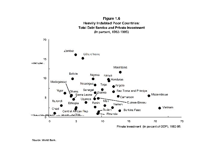
l Figure 1. 6: negative relationship between debt burden and private investment.

Empirical Evidence l General empirical formation of a private investment function : (IP/y) = H ( y, c. K, LP/P, R*, IGI, IGO, z, z , , , D*/y) IP/y: ratio of private investment to output; y: income accelerator effect (captured by changes in output); c. K: user cost of capital; LP/P: credit rationing (captured by the real stock of bank credit to the private sector);

R*: foreign exchange constraint (measured by country's level of foreign reserves); public investment, consists of investment in infrastructure, IGI, and other investments, IGO, with the former variable expected to have a positive effect and the second an ambiguous effect; z: real exchange rate, (has in general an ambiguous effect); macroeconomic instability, captured by the variability of the real exchange rate, z , the level of inflation, , and the variability of inflation, ; D*/y: ratio of foreign debt to output.

Oshikoya (1994) l l l Analysis of the determinants of private investment during the 1970 s and 1980 s in eight African countries: four middle-income countries and four low-income countries. Results: Changes in real output (accelerator effect): significant and positive impact on private investment only in low-income countries. Public investment: positively related to private investment in both groups; stronger complementarity effect in middle-income countries.

l l Real exchange rate: positive and significant effect in middle-income countries; negative effect in lowincome countries. Inflation rate: strong and unambiguously negative impact in low-income countries; positive and significant effect in middle-income countries. Debt service ratio: strong, negative effect on private investment in both country groups. Macroeconomic uncertainty and instability: (coefficients of variation of real output growth and real exchange rate): negative effect on investment during the 1980 s.

Hadjimichael and Ghura (1995) l l For Sub-Saharan Africa. Results: Public and private investment are complementary. Lower inflation and real exchange rate variability promote private investment. A high debt burden has an adverse effect on investment.

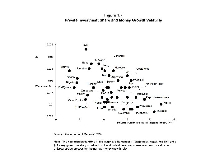
Other Empirical Studies l l l Servén (1997, 1998): robust negative effect of macroeconomic uncertainty on investment, particularly when uncertainty is measured by the real exchange rate. Aizenman and Marion (1999): negative relationship between investment and macroeconomic volatility measures (government consumption as a share of output, nominal money growth and real exchange rate). Figure 1. 7.

l l Cost of waiting is available when as current return on investment exceeds the user cost of capital and equal to this difference. Value of waiting is defined by the irreversible mistake that would be revealed tomorrow if future returns fall short of the user cost of capital.