Chapter 05 CONSUMER COMPARATIVE STATICS Introduction What happens

Chapter 05 CONSUMER COMPARATIVE STATICS

Introduction § What happens to the quantity demanded of any good by a consumer when there is 1. a change in the price of a single good, or 2. a change in income. § We derive individual demand elasticities with respect to prices and income. § We find that while economists generally believe that there is a ‘Law of Demand’ for market demand curves no such law is implied by a consumer’s preference-maximizing behavior for individual demand functions. 2

5. 1 Price and Income Consumption Curves § Individual demand functions, as we have seen in Chapter 4, generally de- pend on three parameters: the prices of the two goods and income. § Changing any one of these at a time enable us to trace the path of utility-maximizing bundles in the commodity space. 3

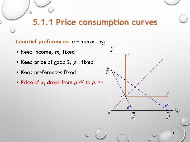
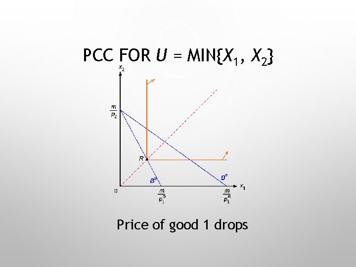
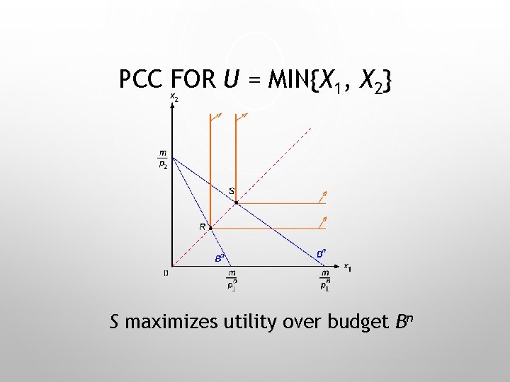
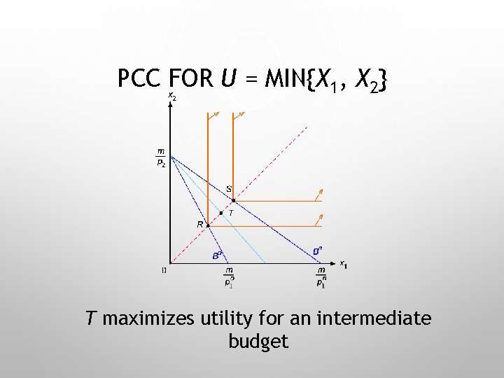
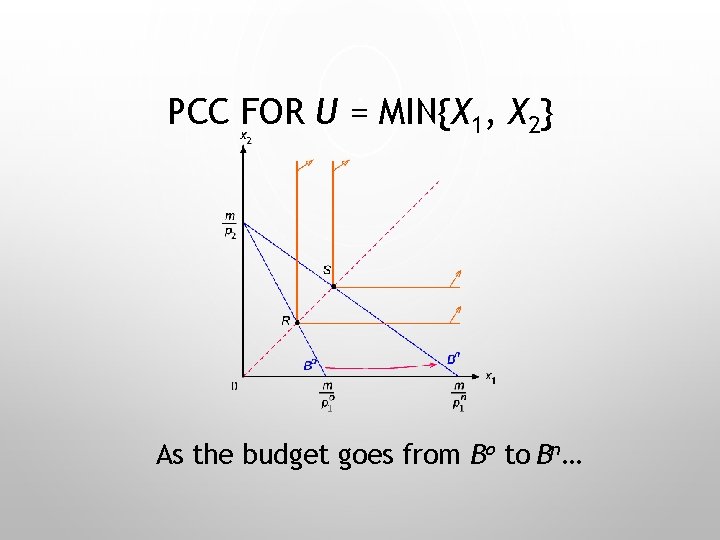
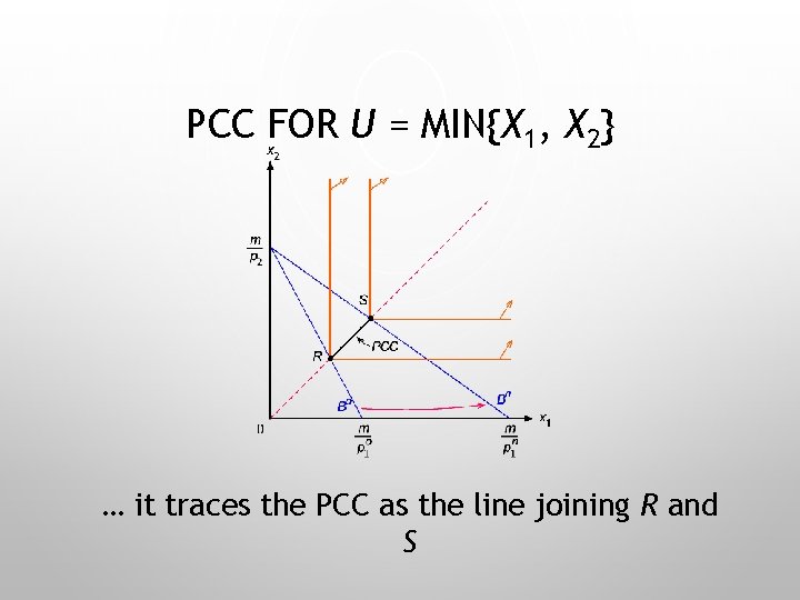
5. 1. 1 Price consumption curves Leontief preferences: u = min{x 1, x 2} § Keep income, m, fixed § Keep price of good 2, p 2, fixed § Keep preferences fixed § Price of x 1 drops from p 1 old to p 1 new 4

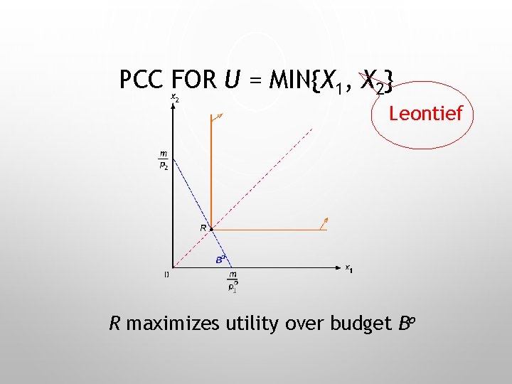
PCC FOR U = MIN{X 1, X 2} Leontief R maximizes utility over budget Bo

PCC FOR U = MIN{X 1, X 2} Price of good 1 drops

PCC FOR U = MIN{X 1, X 2} S maximizes utility over budget Bn

PCC FOR U = MIN{X 1, X 2} T maximizes utility for an intermediate budget

PCC FOR U = MIN{X 1, X 2} As the budget goes from Bo to Bn…

PCC FOR U = MIN{X 1, X 2} … it traces the PCC as the line joining R and S

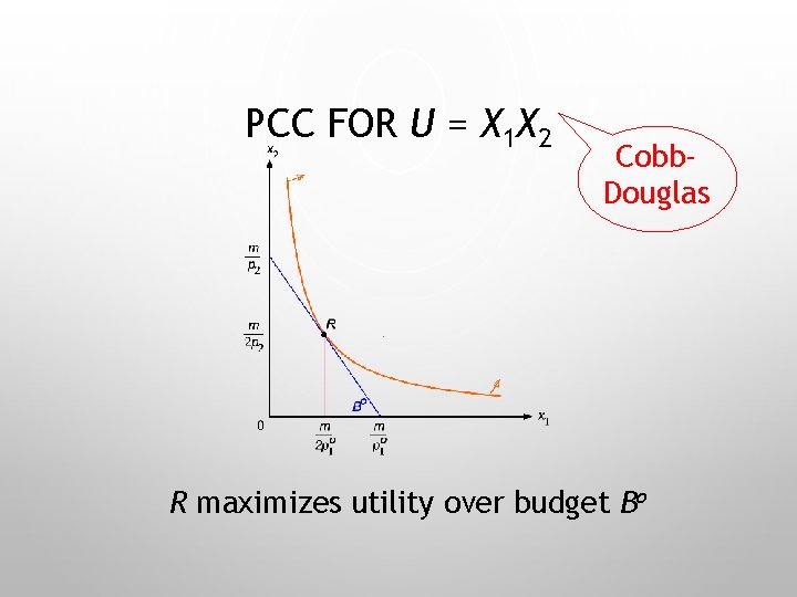
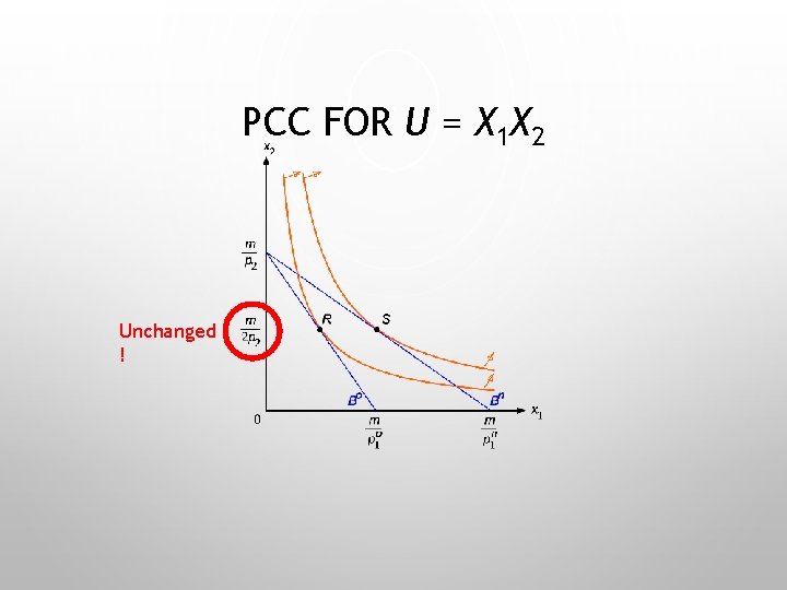
PCC FOR U = X 1 X 2 Cobb. Douglas R maximizes utility over budget Bo

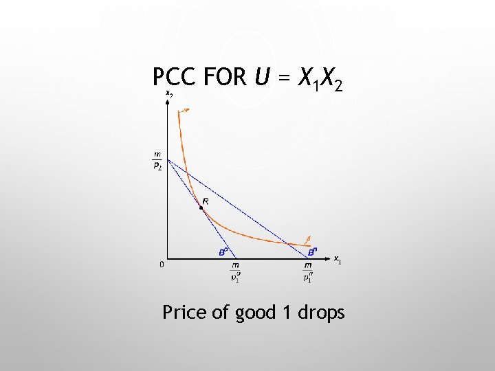
PCC FOR U = X 1 X 2 Price of good 1 drops

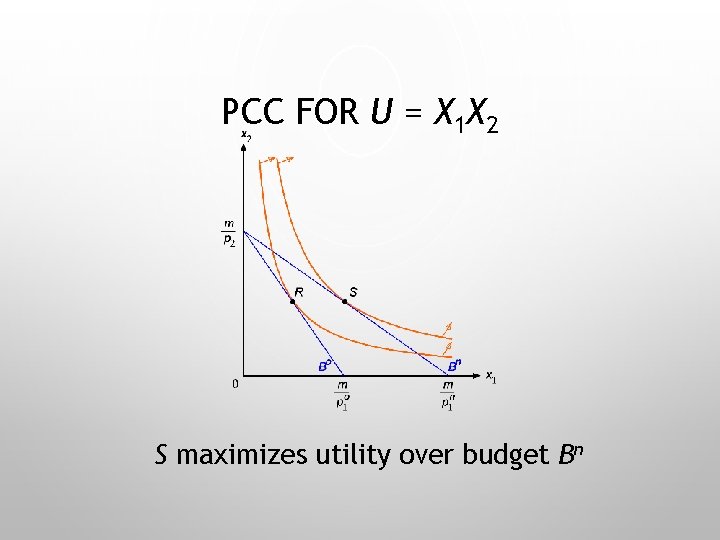
PCC FOR U = X 1 X 2 S maximizes utility over budget Bn

PCC FOR U = X 1 X 2 Unchanged !

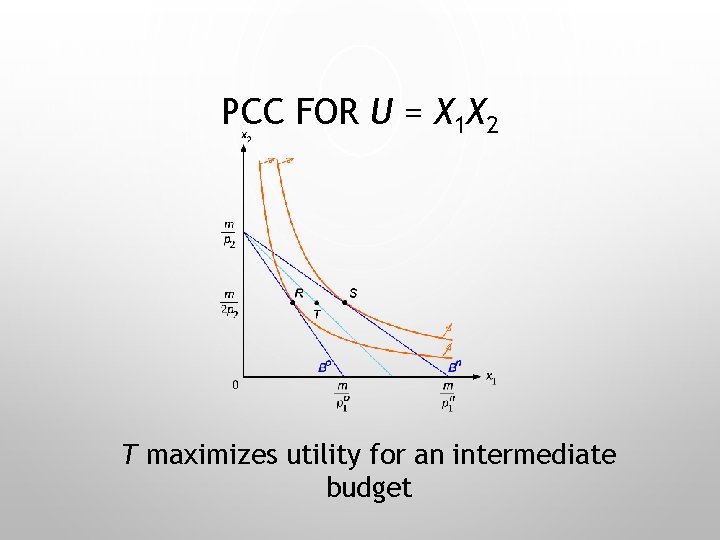
PCC FOR U = X 1 X 2 T maximizes utility for an intermediate budget

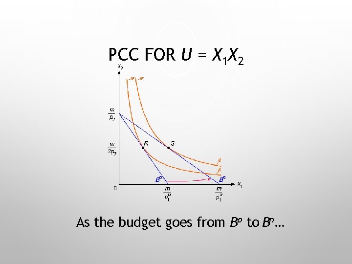
PCC FOR U = X 1 X 2 As the budget goes from Bo to Bn…

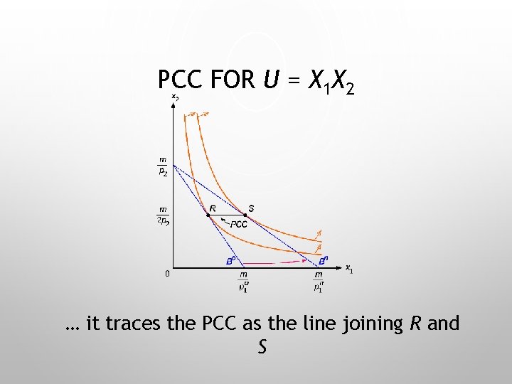
PCC FOR U = X 1 X 2 … it traces the PCC as the line joining R and S

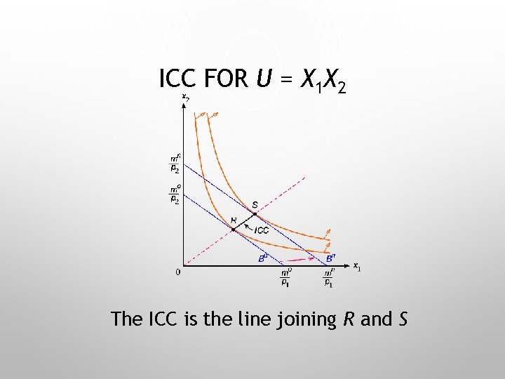
INCOME CONSUMPTION CURVE (ICC) Keeping everything else fixed, how do the utilitymaximizing bundles change as income changes? • • Keep price of good 1, p 1, fixed Keep price of good 2, p 2, fixed Keep preferences fixed Suppose income increases from mold to mnew

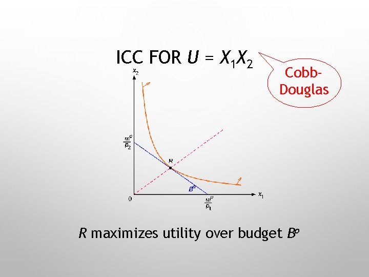
ICC FOR U = X 1 X 2 Cobb. Douglas R maximizes utility over budget Bo

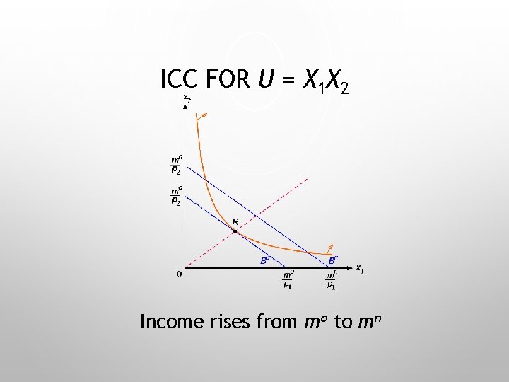
ICC FOR U = X 1 X 2 Income rises from mo to mn

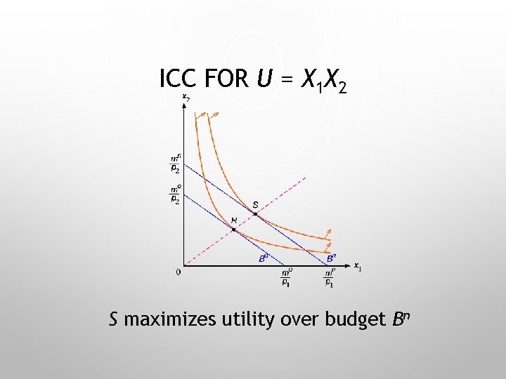
ICC FOR U = X 1 X 2 S maximizes utility over budget Bn

ICC FOR U = X 1 X 2 The ICC is the line joining R and S

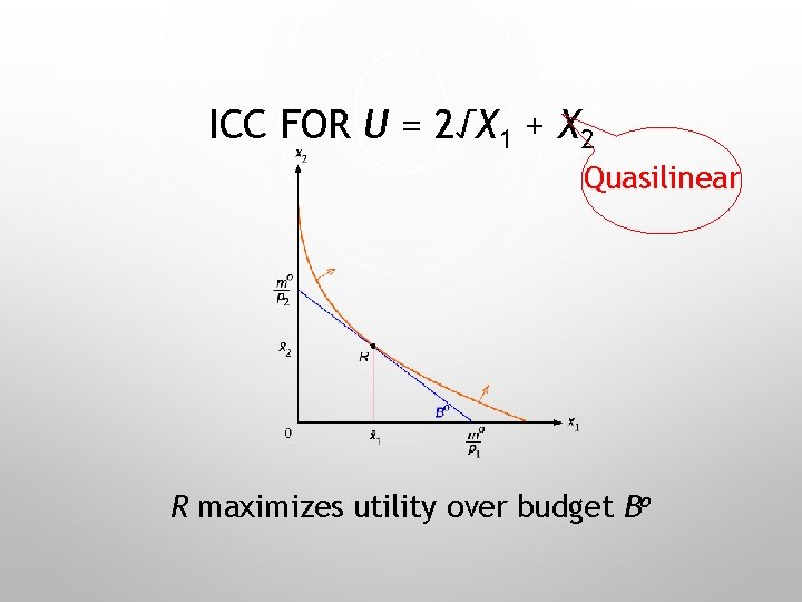
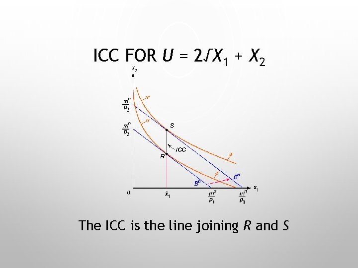
ICC FOR U = 2√X 1 + X 2 Quasilinear R maximizes utility over budget Bo

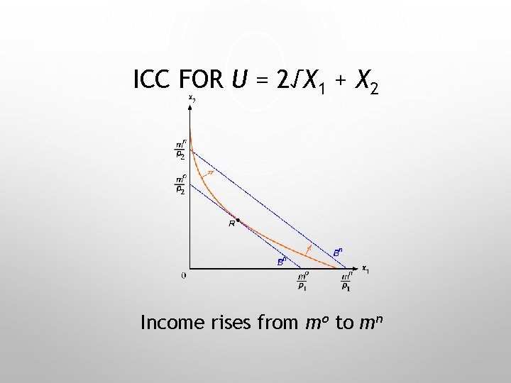
ICC FOR U = 2√X 1 + X 2 Income rises from mo to mn

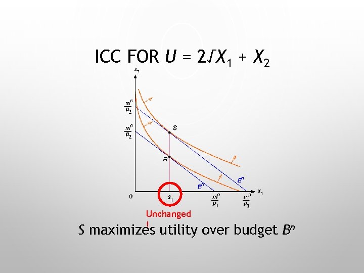
ICC FOR U = 2√X 1 + X 2 Unchanged ! S maximizes utility over budget Bn

ICC FOR U = 2√X 1 + X 2 The ICC is the line joining R and S

INDIVIDUAL DEMAND ELASTICITIES Keeping everything else fixed, what is a consumer’s demand elasticity when • its own price changes? Own-price elasticity of demand • when the price of another good changes? Cross-price elasticity of demand • when income changes? Income elasticity of demand

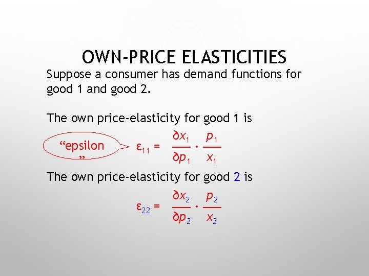
OWN-PRICE ELASTICITIES Suppose a consumer has demand functions for good 1 and good 2. The own price-elasticity for ∂x 1. “epsilon ε 11 = ∂p 1 ” The own price-elasticity for ∂x 2. ε 22 = ∂p 2 good 1 is p 1 x 1 good 2 is p 2 x 2

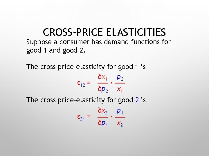
CROSS-PRICE ELASTICITIES Suppose a consumer has demand functions for good 1 and good 2. The cross price-elasticity for good 1 is ∂x 1 p 2. ε 12 = ∂p 2 x 1 The cross price-elasticity for good 2 is ∂x 2 p 1. ε 21 = ∂p 1 x 2

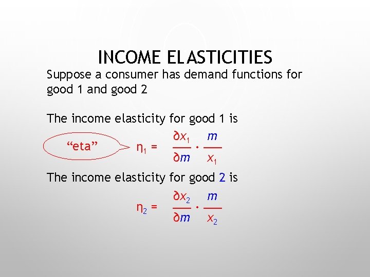
INCOME ELASTICITIES Suppose a consumer has demand functions for good 1 and good 2 The income elasticity for good 1 is ∂x 1 m. “eta” η 1 = ∂m x 1 The income elasticity for good 2 is ∂x 2 m. η 2 = ∂m x 2

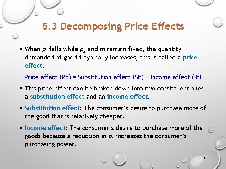
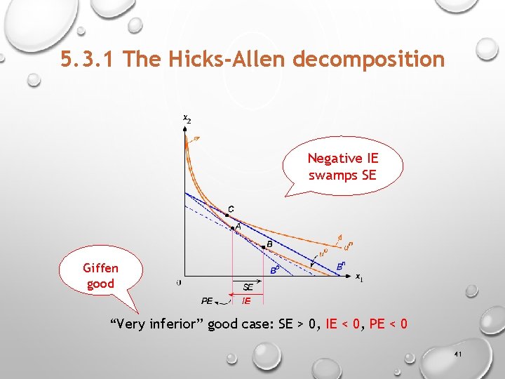
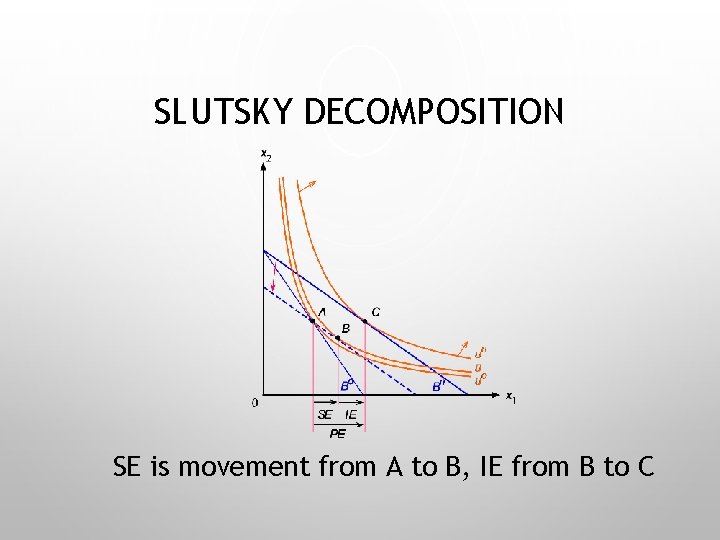
5. 3 Decomposing Price Effects § When p 1 falls while p 2 and m remain fixed, the quantity demanded of good 1 typically increases; this is called a price effect. Price effect (PE) = Substitution effect (SE) + Income effect (IE) § This price effect can be broken down into two constituent ones, a substitution effect and an income effect. § Substitution effect: The consumer’s desire to purchase more of the good that is relatively cheaper. § Income effect: The consumer’s desire to purchase more of the goods because a reduction in p 1 increases the consumer’s purchasing power. 31

5. 3 Decomposing Price Effects § There are two ways of decomposing this price effect: Ø One associated with Sir John Hicks and Sir Roy Allen, Ø and the other with Evgeny (Eugen) Slutsky. 32

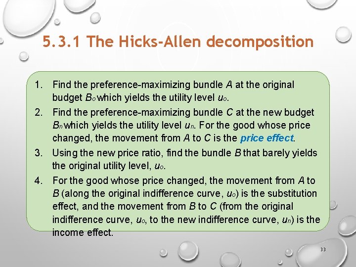
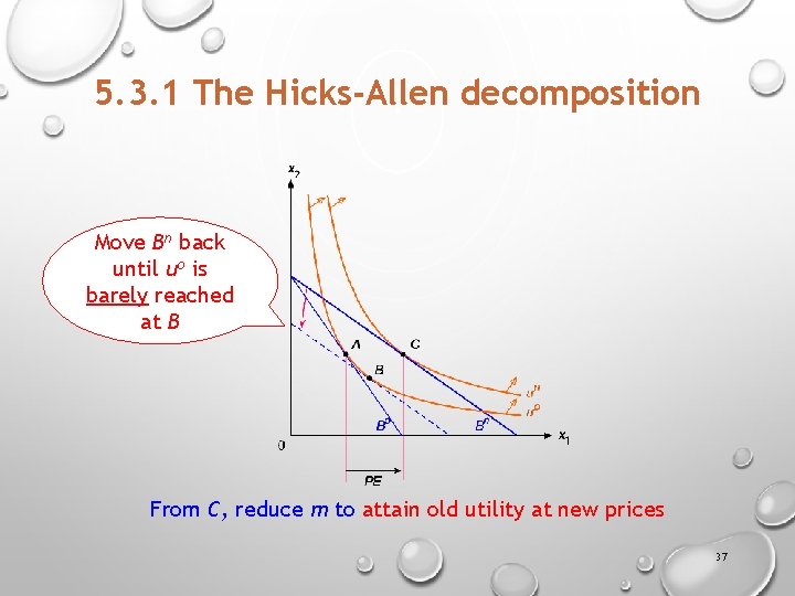
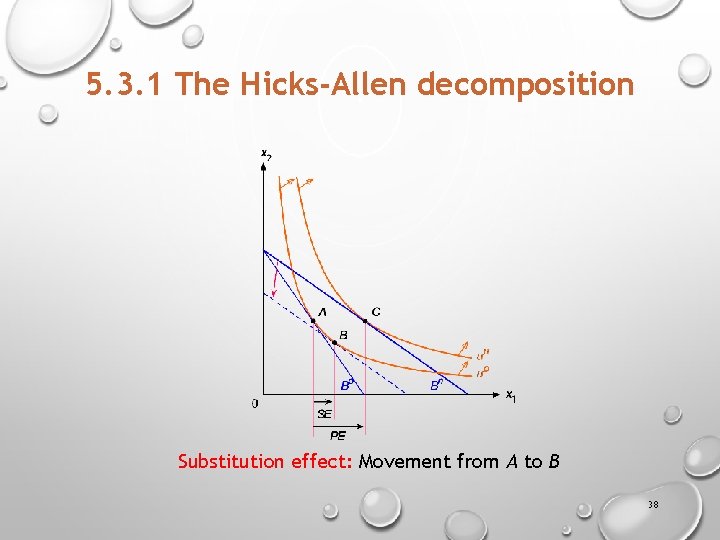
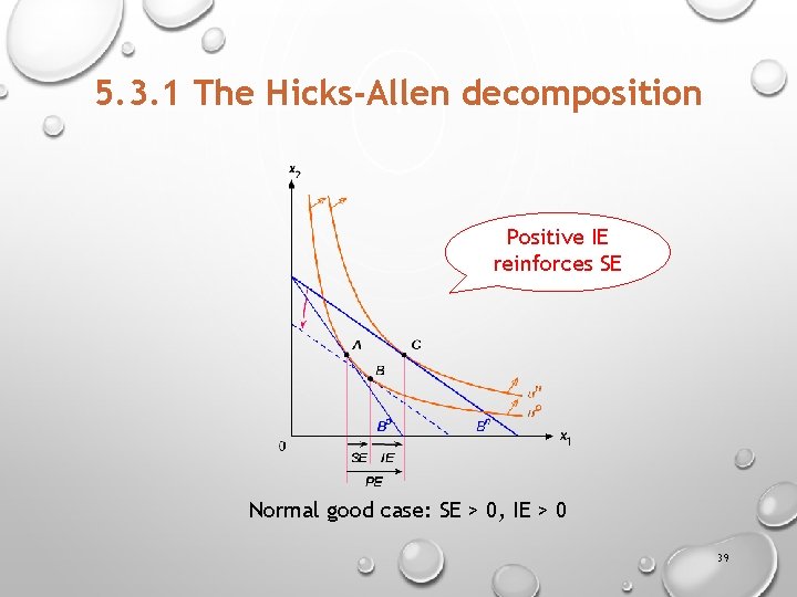
5. 3. 1 The Hicks-Allen decomposition 1. Find the preference-maximizing bundle A at the original budget Bo which yields the utility level uo. 2. Find the preference-maximizing bundle C at the new budget Bn which yields the utility level un. For the good whose price changed, the movement from A to C is the price effect. 3. Using the new price ratio, find the bundle B that barely yields the original utility level, uo. 4. For the good whose price changed, the movement from A to B (along the original indifference curve, uo) is the substitution effect, and the movement from B to C (from the original indifference curve, uo, to the new indifference curve, un) is the income effect. 33

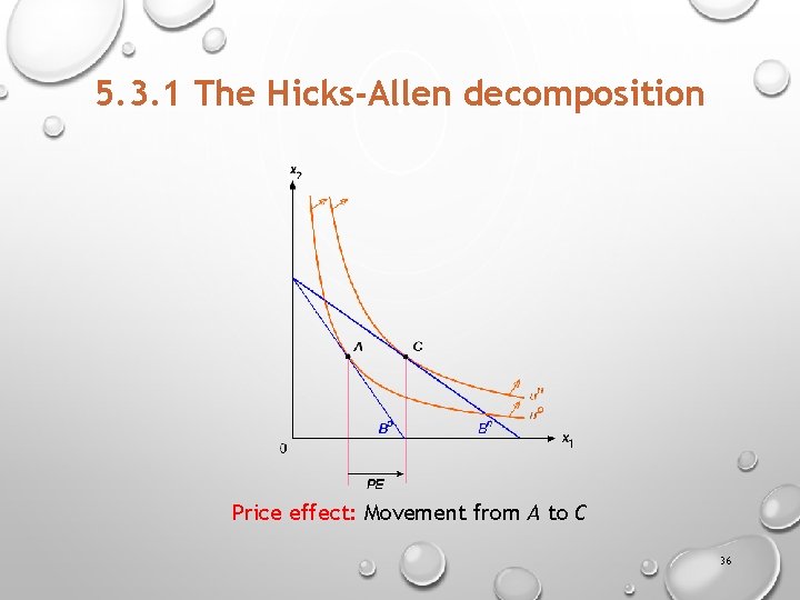
5. 3. 1 The Hicks-Allen decomposition Bundle A maximizes utility over budget Bo 34

5. 3. 1 The Hicks-Allen decomposition Bundle C maximizes utility over budget Bn 35

5. 3. 1 The Hicks-Allen decomposition Price effect: Movement from A to C 36

5. 3. 1 The Hicks-Allen decomposition Move Bn back until uo is barely reached at B From C, reduce m to attain old utility at new prices 37

5. 3. 1 The Hicks-Allen decomposition Substitution effect: Movement from A to B 38

5. 3. 1 The Hicks-Allen decomposition Positive IE reinforces SE Normal good case: SE > 0, IE > 0 39

5. 3. 1 The Hicks-Allen decomposition Negative IE dampens SE “Slightly” inferior good case: SE > 0, IE < 0, PE > 0 40

5. 3. 1 The Hicks-Allen decomposition Negative IE swamps SE Giffen good “Very inferior” good case: SE > 0, IE < 0, PE < 0 41

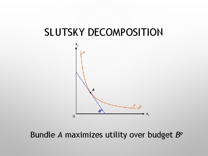
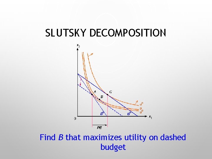
SLUTSKY DECOMPOSITION Bundle A maximizes utility over budget Bo

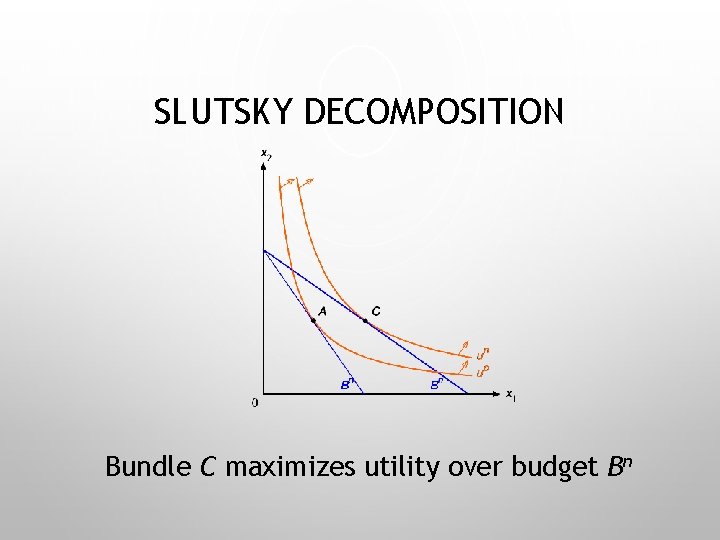
SLUTSKY DECOMPOSITION Bundle C maximizes utility over budget Bn

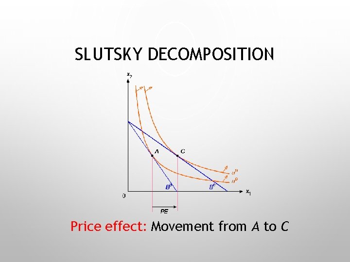
SLUTSKY DECOMPOSITION Price effect: Movement from A to C

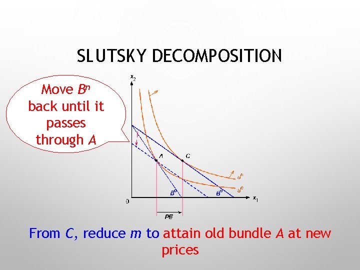
SLUTSKY DECOMPOSITION Move Bn back until it passes through A From C, reduce m to attain old bundle A at new prices

SLUTSKY DECOMPOSITION Find B that maximizes utility on dashed budget

SLUTSKY DECOMPOSITION SE is movement from A to B, IE from B to C