Chap 5 ARIMA Model Ani Shabri Department of

Chap 5: ARIMA Model Ani Shabri Department of Mathematical Sciences, Faculty of Science, Universiti Teknologi Malaysia, 81310 UTM Johor Bahru, Malaysia ani@utm. my Jun 8, 2014 1

Chap 5: ARIMA models Outline: • Introduction to Box-Jenkins methodology • Box-Jenkins methodology procedure • Stationarity • Transformations to achieve stationary • Models for stationary time series • Identification ARIMA models • Parameter estimation technique • Diagnostics Checking • Forecasting 2

Introduction to Box-Jenkins methodology • Box-Jenkins (BJ) methodology or Autoregressive Integrated Moving Average (ARIMA) models are a class of linear models that is capable of representing stationary as well as non-stationary time series. • The BJ methodology refers to a set of procedures for identifying, fitting, estimating and checking ARIMA models with time series data. Forecast follow directly from the form of fitted model. • The BJ methodology aims to obtain a model that is parsimony. Parsimony referred a model has the smallest number of parameters needed to adequately fit the patterns in the data observed. 3

Box-Jenkins methodology procedure • Stationary: Stationary is a fundamental property underlying for ARIMA model. In this step, non-stationary to achieve stationary series usually by taking first and second difference of the data. • Identification: When the data are confirmed stationary, one may proceed to tentative identification of models through visual inspection of both the autocorrelation function (ACF) and partial autocorrelation function (PACF). • Estimation: Determine coefficients and estimate of the ARIMA model using various techniques such as the least squares, moment and maximum likelihood methods. • Diagnostics: Having estimated the coefficients, the model is then tested for its adequacy. Test statistics, ACFs and PACFs of residuals were used to verify whether the model is valid. If valid then use the decided model, otherwise repeat the steps of Identification, Estimation and Diagnostics. • Forecast: Once the model’s fitness has been confirmed, the model then ready to be used to generate the forecasts for future value. 4

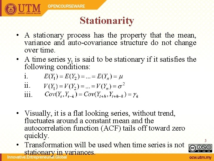
Stationarity • A stationary process has the property that the mean, variance and auto-covariance structure do not change over time. • A time series yt is said to be stationary if it satisfies the following conditions: i. iii. • Visually, it is a flat looking series, without trend, fluctuates around a constant mean and the autocorrelation function (ACF) tails off toward zero quickly. • Transformation will be used when time series is not stationary in variances. 5

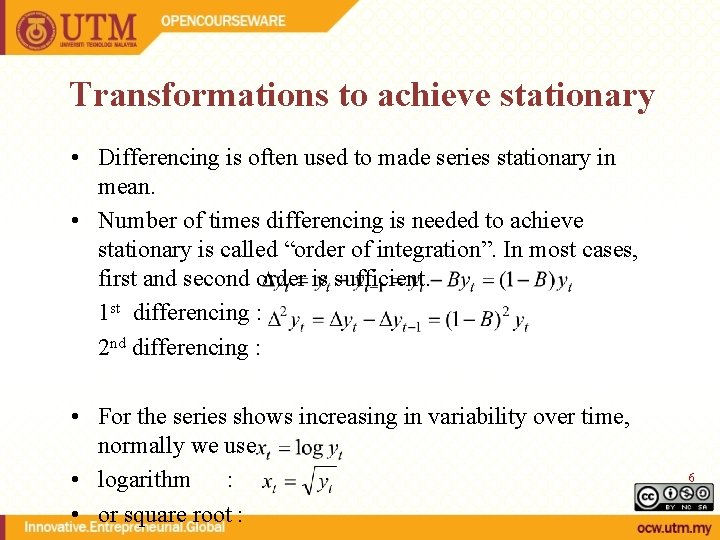
Transformations to achieve stationary • Differencing is often used to made series stationary in mean. • Number of times differencing is needed to achieve stationary is called “order of integration”. In most cases, first and second order is sufficient. 1 st differencing : 2 nd differencing : • For the series shows increasing in variability over time, normally we use • logarithm : • or square root : 6

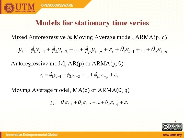
Models for stationary time series Mixed Autoregressive & Moving Average model, ARMA(p, q) Autoregressive model, AR(p) or ARMA(p, 0) Moving Average model, MA(q) or ARMA(0, q) 7

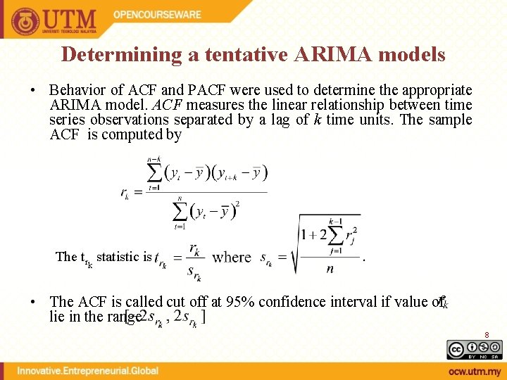
Determining a tentative ARIMA models • Behavior of ACF and PACF were used to determine the appropriate ARIMA model. ACF measures the linear relationship between time series observations separated by a lag of k time units. The sample ACF is computed by The trk statistic is • The ACF is called cut off at 95% confidence interval if value of lie in the range 8

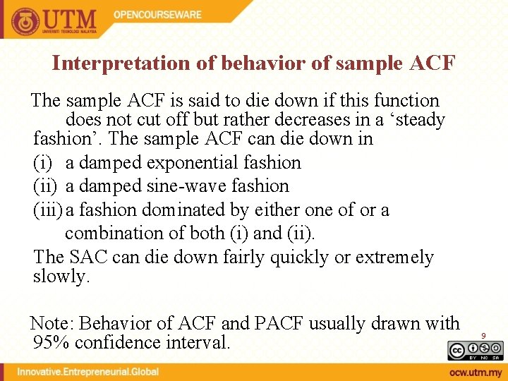
Interpretation of behavior of sample ACF The sample ACF is said to die down if this function does not cut off but rather decreases in a ‘steady fashion’. The sample ACF can die down in (i) a damped exponential fashion (ii) a damped sine-wave fashion (iii) a fashion dominated by either one of or a combination of both (i) and (ii). The SAC can die down fairly quickly or extremely slowly. Note: Behavior of ACF and PACF usually drawn with 95% confidence interval. 9

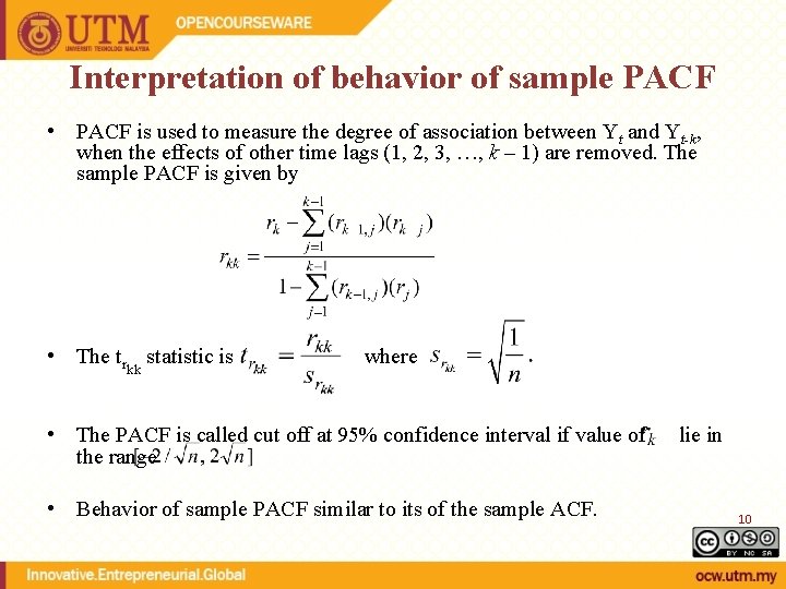
Interpretation of behavior of sample PACF • PACF is used to measure the degree of association between Yt and Yt-k, when the effects of other time lags (1, 2, 3, …, k – 1) are removed. The sample PACF is given by • The trkk statistic is where • The PACF is called cut off at 95% confidence interval if value of the range • Behavior of sample PACF similar to its of the sample ACF. lie in 10

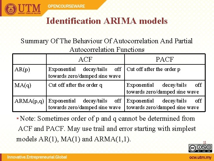
Identification ARIMA models Summary Of The Behaviour Of Autocorrelation And Partial Autocorrelation Functions ACF PACF AR(p) Exponential decay/tails off towards zero/damped sine wave Cut off after the order p MA(q) Cut off after the order q Exponential decay/tails off towards zero/damped sine wave ARMA(p, q) Exponential decay/tails off towards zero/damped sine wave * Note: Sometimes order of p and q cannot be determined from ACF and PACF. May use trail and error starting with simplest models AR(1), MA(1) and ARMA(1, 1). 11

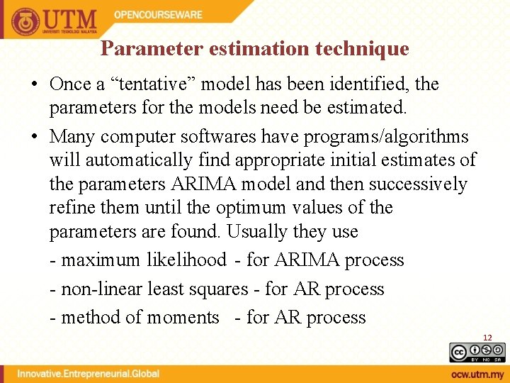
Parameter estimation technique • Once a “tentative” model has been identified, the parameters for the models need be estimated. • Many computer softwares have programs/algorithms will automatically find appropriate initial estimates of the parameters ARIMA model and then successively refine them until the optimum values of the parameters are found. Usually they use - maximum likelihood - for ARIMA process - non-linear least squares - for AR process - method of moments - for AR process 12

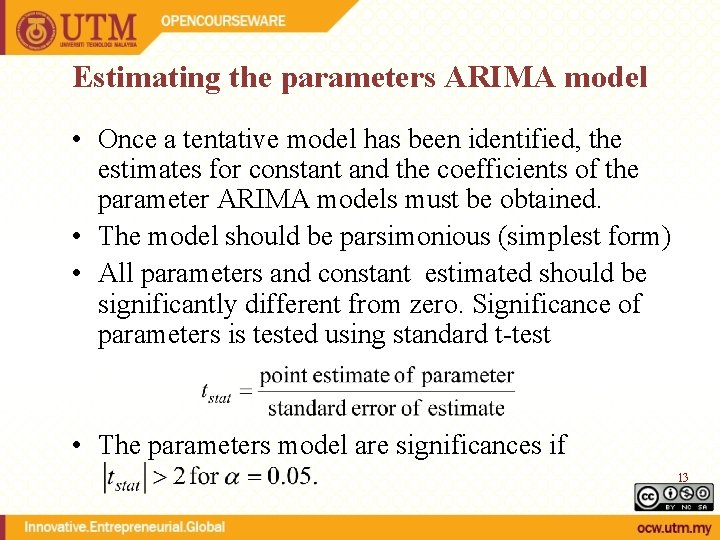
Estimating the parameters ARIMA model • Once a tentative model has been identified, the estimates for constant and the coefficients of the parameter ARIMA models must be obtained. • The model should be parsimonious (simplest form) • All parameters and constant estimated should be significantly different from zero. Significance of parameters is tested using standard t-test • The parameters model are significances if 13

Diagnostics Checking In the model-building process, if an ARIMA(p, d, q) model is chosen (based on the ACFs and PACFs), some checks on the model adequacy are required. A residual analysis is usually based on the fact that the residuals of an adequate model should be approximately white noise. Basically, a model is adequate if the residuals nearly the properties white noise process, i. e. the errors § constant on variances § Independent § normally distributed with zero means and variance σ2 14

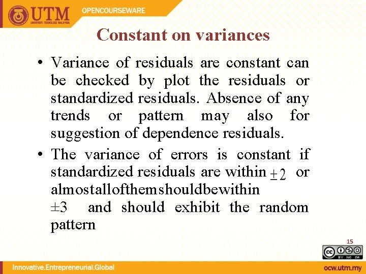
Constant on variances • Variance of residuals are constant can be checked by plot the residuals or standardized residuals. Absence of any trends or pattern may also for suggestion of dependence residuals. • The variance of errors is constant if standardized residuals are within or almost all of them should be within ± 3 and should exhibit the random pattern 15

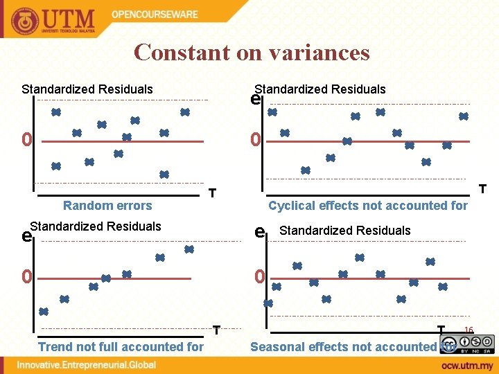
Constant on variances Standardized Residuals e 0 0 Random errors Standardized Residuals T T Standardized Residuals Cyclical effects not accounted for e e 0 0 T Trend not full accounted for Standardized Residuals T Seasonal effects not accounted for 16

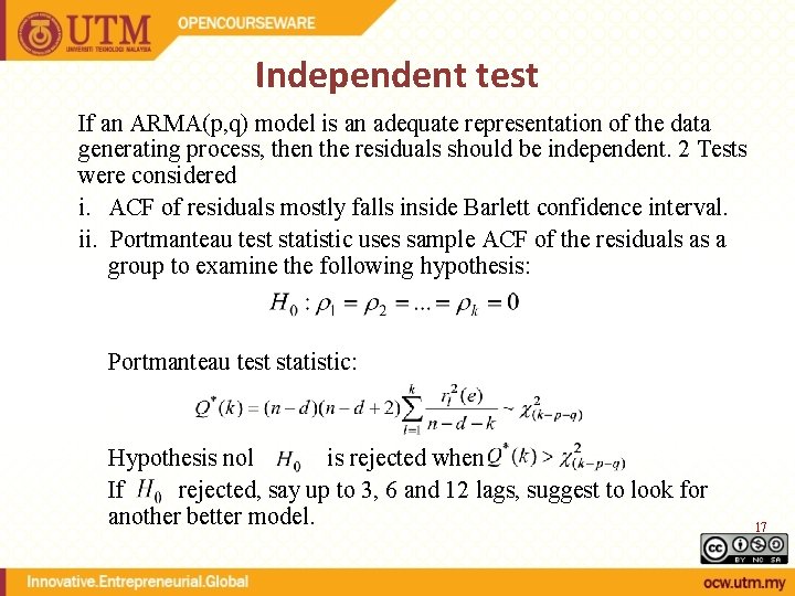
Independent test If an ARMA(p, q) model is an adequate representation of the data generating process, then the residuals should be independent. 2 Tests were considered i. ACF of residuals mostly falls inside Barlett confidence interval. ii. Portmanteau test statistic uses sample ACF of the residuals as a group to examine the following hypothesis: Portmanteau test statistic: Hypothesis nol is rejected when If rejected, say up to 3, 6 and 12 lags, suggest to look for another better model. 17

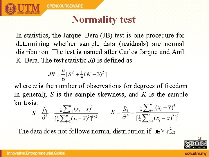
Normality test In statistics, the Jarque–Bera (JB) test is one procedure for determining whether sample data (residuals) are normal distribution. The test is named after Carlos Jarque and Anil K. Bera. The test statistic JB is defined as where n is the number of observations (or degrees of freedom in general); S is the sample skewness, and K is the sample kurtosis: The data does not follows normal distribution if JB 18

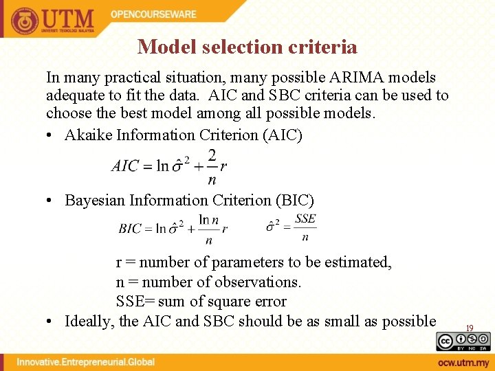
Model selection criteria In many practical situation, many possible ARIMA models adequate to fit the data. AIC and SBC criteria can be used to choose the best model among all possible models. • Akaike Information Criterion (AIC) • Bayesian Information Criterion (BIC) r = number of parameters to be estimated, n = number of observations. SSE= sum of square error • Ideally, the AIC and SBC should be as small as possible 19

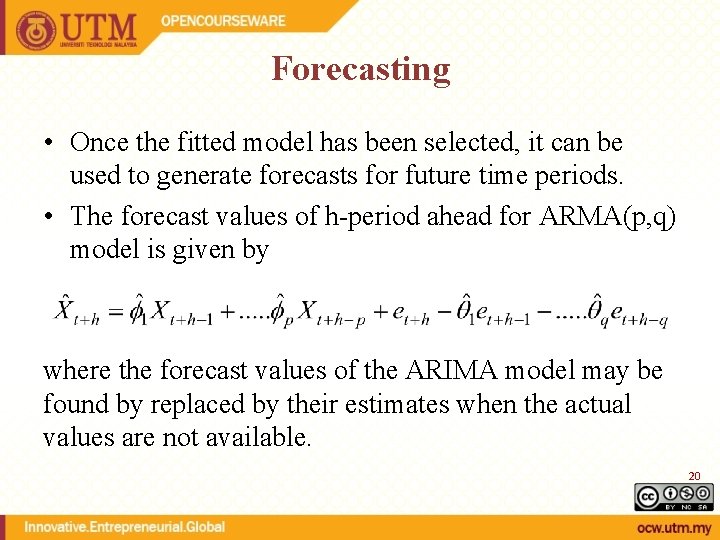
Forecasting • Once the fitted model has been selected, it can be used to generate forecasts for future time periods. • The forecast values of h-period ahead for ARMA(p, q) model is given by where the forecast values of the ARIMA model may be found by replaced by their estimates when the actual values are not available. 20

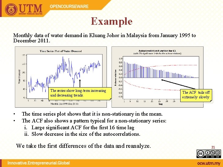
Example Monthly data of water demand in Kluang Johor in Malaysia from January 1995 to December 2011. The series show long-term increasing and decreasing trends. • • The ACF tails off extremely slowly The time series plot shows that it is non-stationary in the mean. The ACF also shows a pattern typical for a non-stationary series: i. Large significant ACF for the first 16 time lag ii. Slow decrease in the size of the autocorrelations. We take the first differences of the data and reanalyze. 21

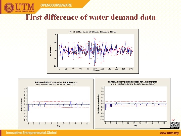
First difference of water demand data 22

Example • The plot and ACF (cuts off quickly) of the 1 st difference of water demand suggests the series is stationary. • Based on ACF and PACF, 3 tentative models are identified i. ARIMA(0, 1, 1)-ACF cuts off after lag 1 and PACF shows a exponential decay ii. ARIMA (2, 1, 1)-ACF follows a damped cycle and PACF cuts off after lag 2. iii. ARIMA(1, 1, 1)-ACF and PACF decay exponentially. 23

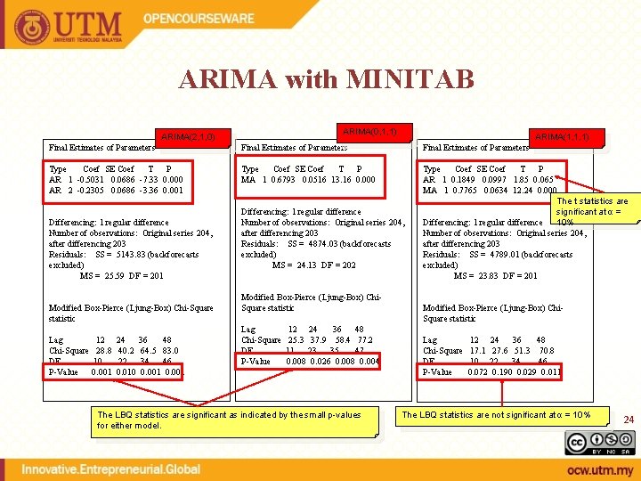
ARIMA with MINITAB ARIMA(0, 1, 1) ARIMA(2, 1, 0) ARIMA(1, 1, 1) Final Estimates of Parameters Type Coef SE Coef T P AR 1 -0. 5031 0. 0686 -7. 33 0. 000 AR 2 -0. 2305 0. 0686 -3. 36 0. 001 Type Coef SE Coef T P MA 1 0. 6793 0. 0516 13. 16 0. 000 Type Coef SE Coef T P AR 1 0. 1849 0. 0997 1. 85 0. 065 MA 1 0. 7765 0. 0634 12. 24 0. 000 The t statistics are significant at α = Differencing: 1 regular difference 10% Number of observations: Original series 204, after differencing 203 Residuals: SS = 4789. 01 (backforecasts excluded) MS = 23. 83 DF = 201 Differencing: 1 regular difference Number of observations: Original series 204, after differencing 203 Residuals: SS = 5143. 83 (backforecasts excluded) MS = 25. 59 DF = 201 Modified Box-Pierce (Ljung-Box) Chi-Square statistic Lag 12 Chi-Square 28. 8 DF 10 P-Value 0. 001 24 36 48 40. 2 64. 5 83. 0 22 34 46 0. 010 0. 001 Differencing: 1 regular difference Number of observations: Original series 204, after differencing 203 Residuals: SS = 4874. 03 (backforecasts excluded) MS = 24. 13 DF = 202 Modified Box-Pierce (Ljung-Box) Chi. Square statistic Lag Chi-Square DF P-Value 12 24 36 48 25. 3 37. 9 58. 4 77. 2 11 23 35 47 0. 008 0. 026 0. 008 0. 004 The LBQ statistics are significant as indicated by the small p-values for either model. Modified Box-Pierce (Ljung-Box) Chi. Square statistic Lag Chi-Square DF P-Value 12 24 36 48 17. 1 27. 6 51. 3 70. 8 10 22 34 46 0. 072 0. 190 0. 029 0. 011 The LBQ statistics are not significant at α = 10% 24

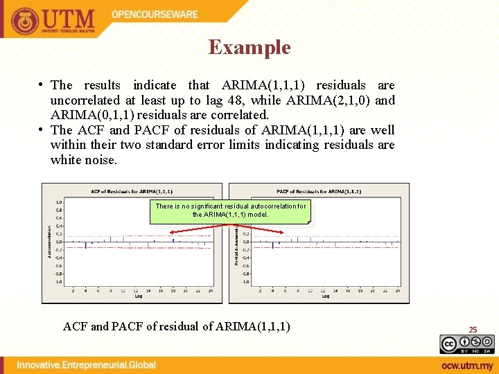
Example • The results indicate that ARIMA(1, 1, 1) residuals are uncorrelated at least up to lag 48, while ARIMA(2, 1, 0) and ARIMA(0, 1, 1) residuals are correlated. • The ACF and PACF of residuals of ARIMA(1, 1, 1) are well within their two standard error limits indicating residuals are white noise. There is no significant residual autocorrelation for the ARIMA(1, 1, 1) model. ACF and PACF of residual of ARIMA(1, 1, 1) 25

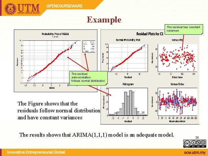
Example The residual has constant variances The residual autocorrelation follows normal distribution The Figure shows that the residuals follow normal distribution and have constant variances The results shows that ARIMA(1, 1, 1) model is an adequate model. 26

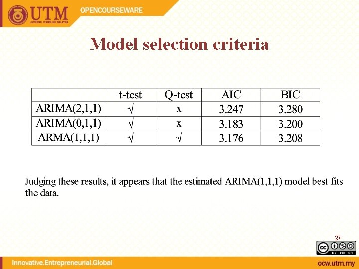
Model selection criteria 27

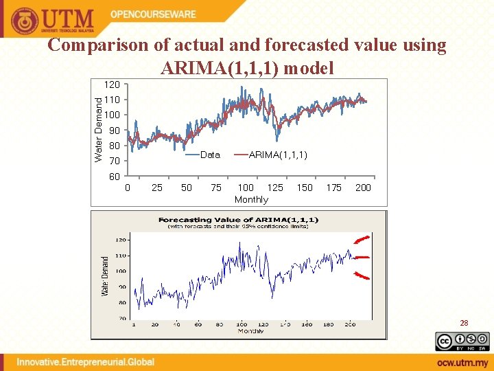
Comparison of actual and forecasted value using ARIMA(1, 1, 1) model Water Demand 120 110 100 90 80 Data 70 ARIMA(1, 1, 1) 60 0 25 50 75 100 125 Monthly 150 175 200 28