Chap 3 String Matching 3 1 String Matching

Chap 3 String Matching 3 - 1

String Matching Problem • A classical and important problem • Searching engines (like Goole and Openfind) • Database (Gen. Bank) 3 - 2

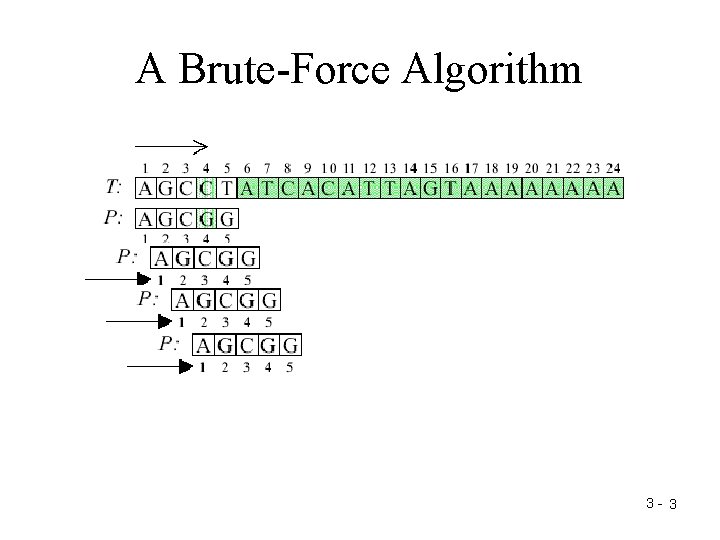
A Brute-Force Algorithm 3 - 3

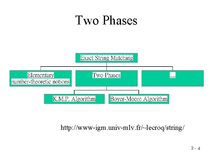
Two Phases http: //www-igm. univ-mlv. fr/~lecroq/string/ 3 - 4

Two Phases • Phase 1：generate an array to indicate the moving direction. • Phase 2：make use of the array to move and match string 3 - 5

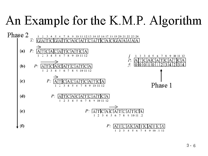
An Example for the K. M. P. Algorithm Phase 2 Phase 1 3 - 6

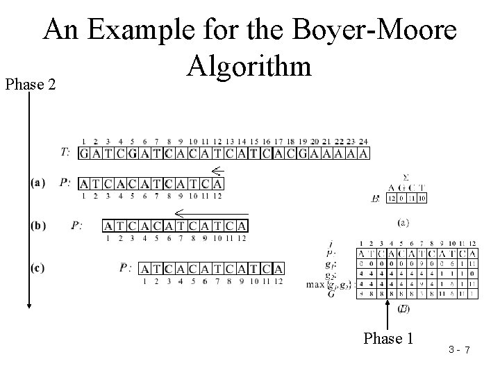
An Example for the Boyer-Moore Algorithm Phase 2 Phase 1 3 - 7

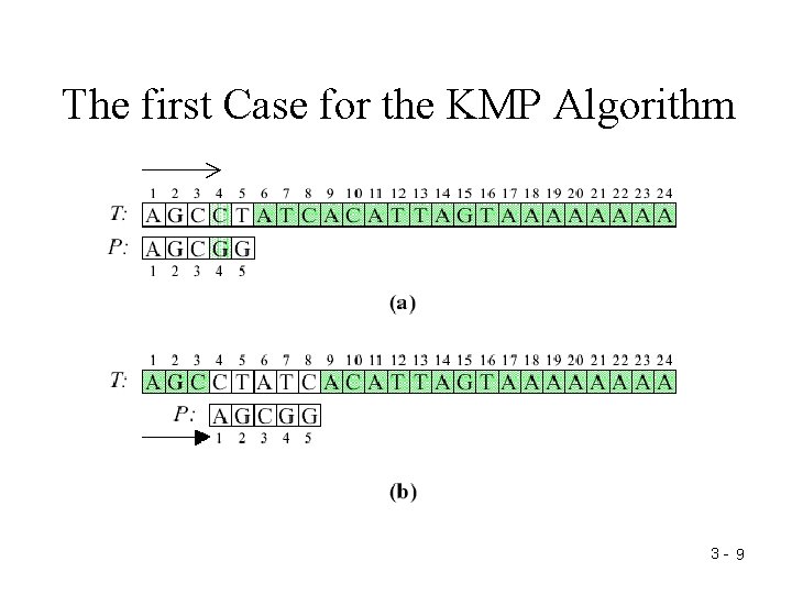
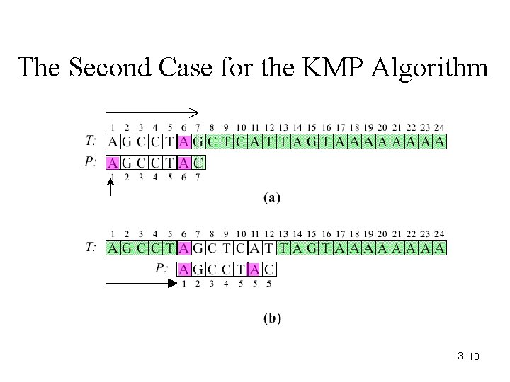
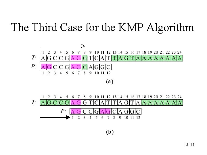
The K. M. P. Algorithm • Proposed by Knuth, Morris and Pratt in 1977. • Three cases to illustrate their idea. 3 - 8

The first Case for the KMP Algorithm 3 - 9

The Second Case for the KMP Algorithm 3 -10

The Third Case for the KMP Algorithm 3 -11

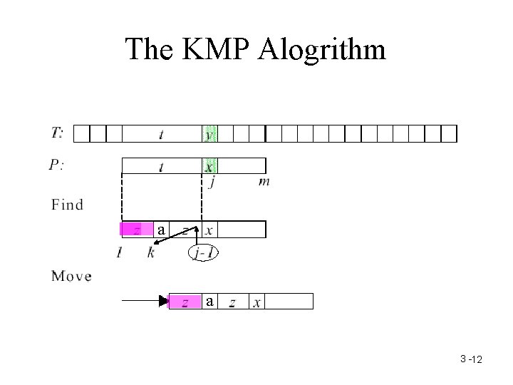
The KMP Alogrithm a a 3 -12

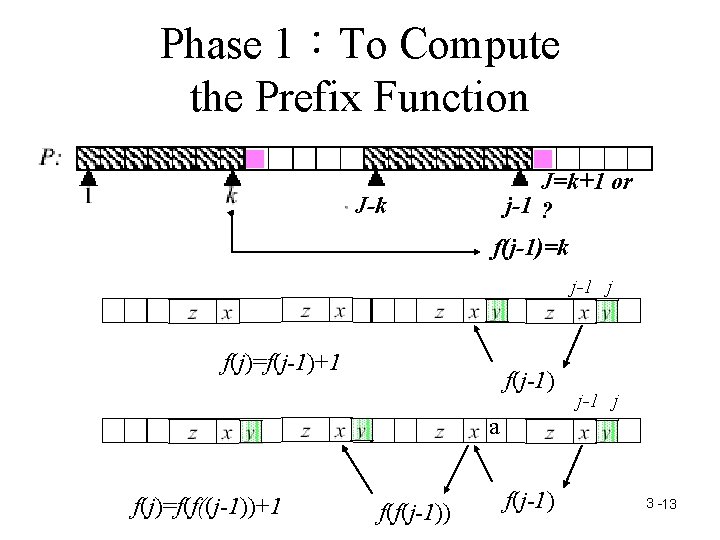
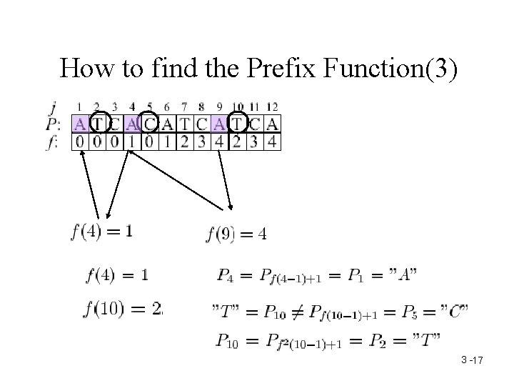
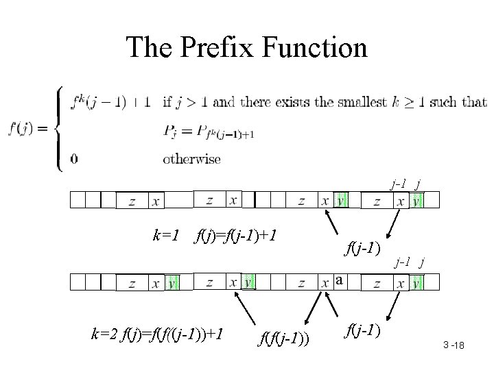
Phase 1：To Compute the Prefix Function J=k+1 or j-1 ? J-k f(j-1)=k j-1 j f(j)=f(j-1)+1 f(j-1) j-1 j a f(j)=f(f((j-1))+1 f(f(j-1)) f(j-1) 3 -13

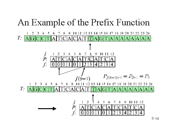
An Example of the Prefix Function 3 -14

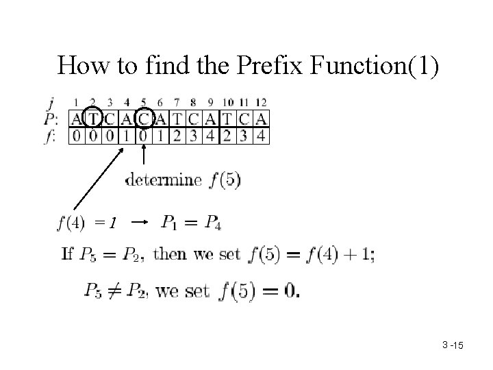
How to find the Prefix Function(1) =1 3 -15

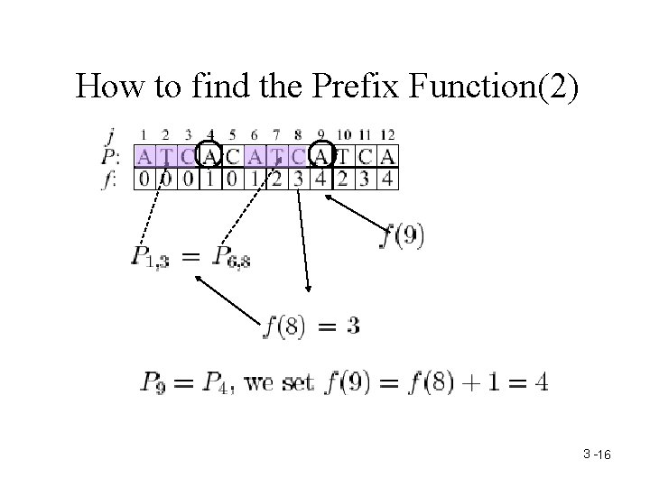
How to find the Prefix Function(2) 3 -16

How to find the Prefix Function(3) 3 -17

The Prefix Function j-1 j k=1 f(j)=f(j-1)+1 f(j-1) j-1 j a k=2 f(j)=f(f((j-1))+1 f(f(j-1)) f(j-1) 3 -18

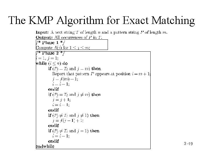
The KMP Algorithm for Exact Matching 3 -19

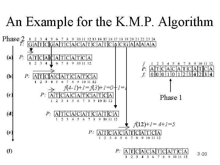
An Example for the K. M. P. Algorithm Phase 2 f(4 -1)+1= f(3)+1=0+1=1 Phase 1 f(12)+1= 4+1=5 3 -20

The analysis of the K. M. P. Algorithm • O(m+n) – O(m) for computing function f – O(n) for searching P 3 -21

An Example for the Boyer-Moore Algorithm Phase 2 Phase 1 3 -22

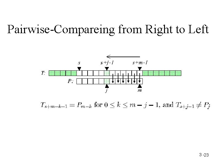
Pairwise-Compareing from Right to Left 3 -23

The Rule of Moving the Window • Bad Character Rule • Good Suffix Rule – Good Suffix Rule 1 – Good Suffix Rule 2 3 -24

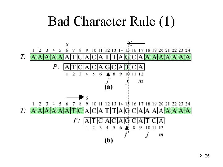
Bad Character Rule (1) 3 -25

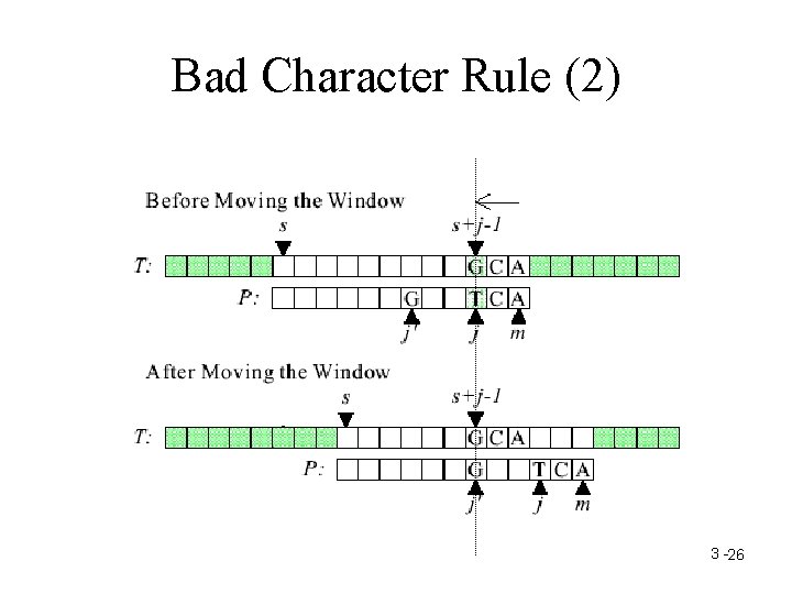
Bad Character Rule (2) 3 -26

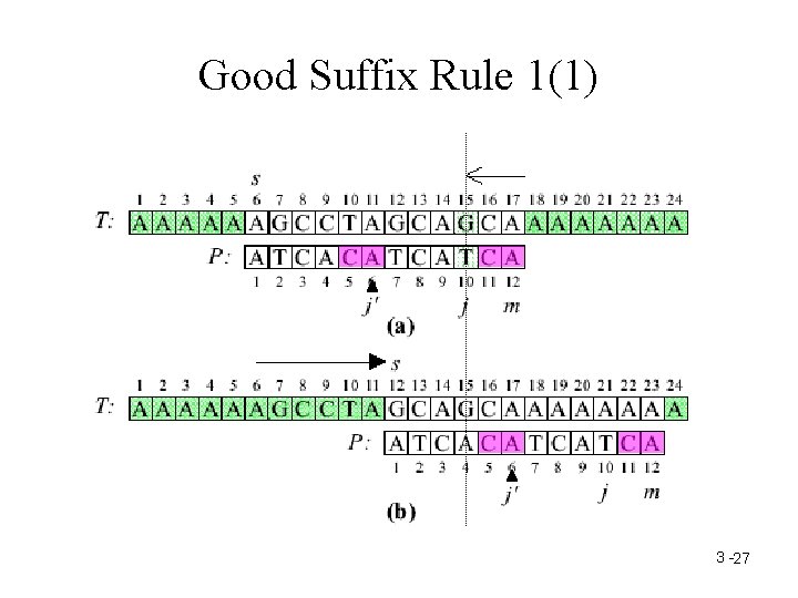
Good Suffix Rule 1(1) 3 -27

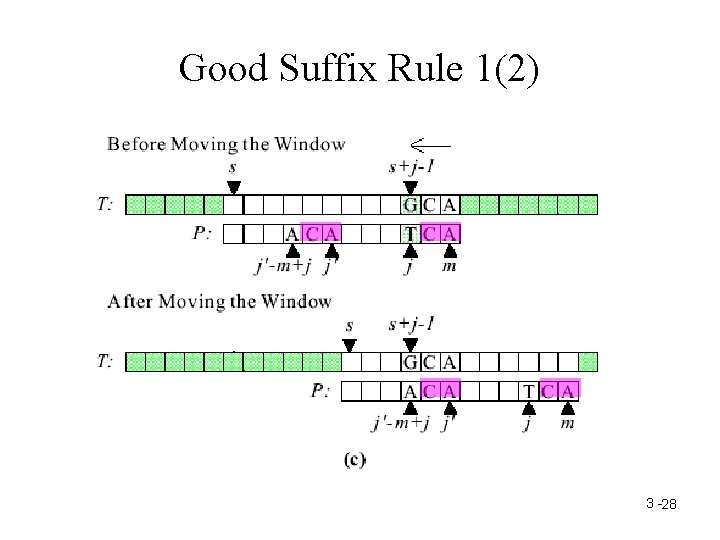
Good Suffix Rule 1(2) 3 -28

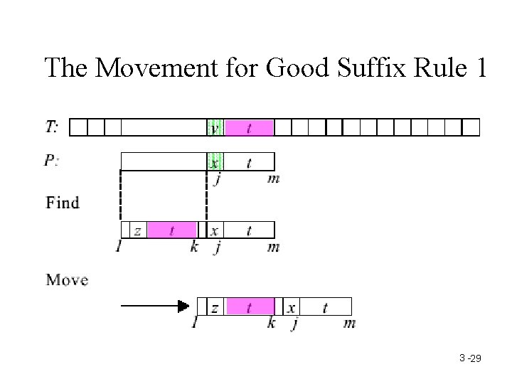
The Movement for Good Suffix Rule 1 3 -29

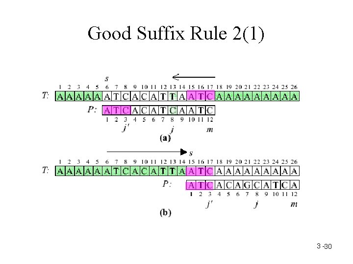
Good Suffix Rule 2(1) 3 -30

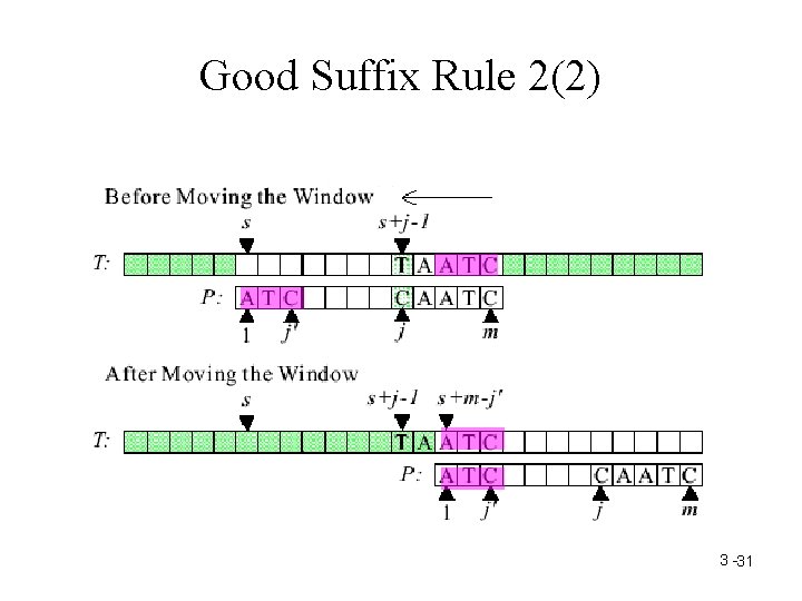
Good Suffix Rule 2(2) 3 -31

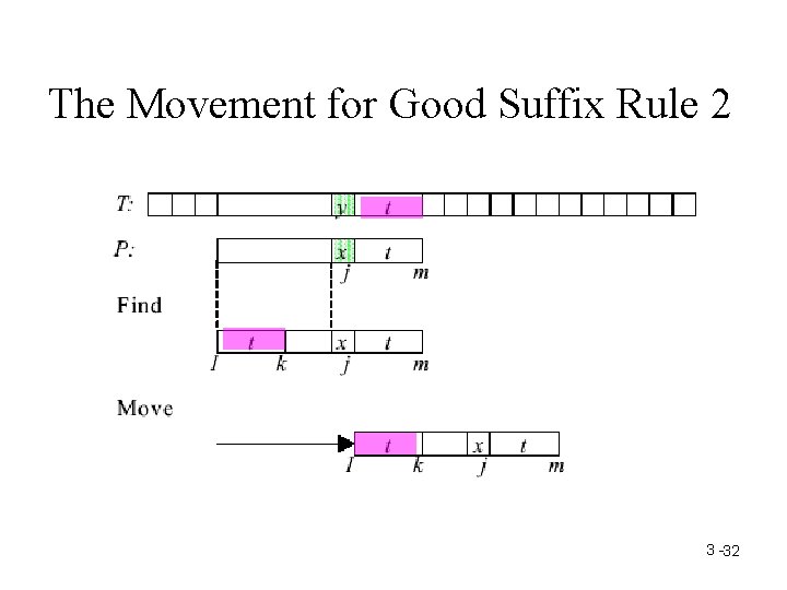
The Movement for Good Suffix Rule 2 3 -32

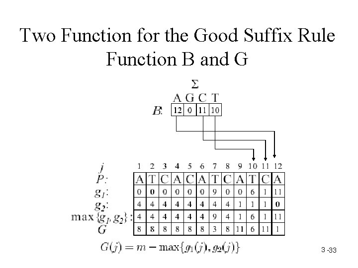
Two Function for the Good Suffix Rule Function B and G (b) 3 -33

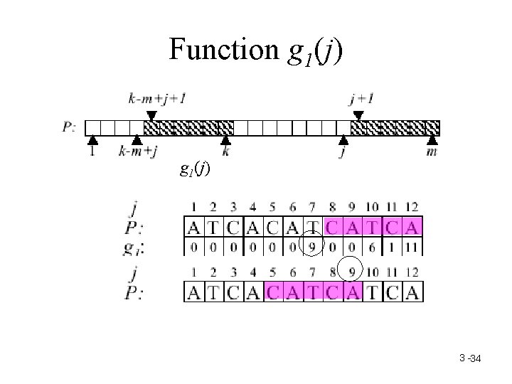
Function g 1(j) 3 -34

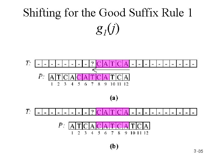
Shifting for the Good Suffix Rule 1 g 1(j) 3 -35

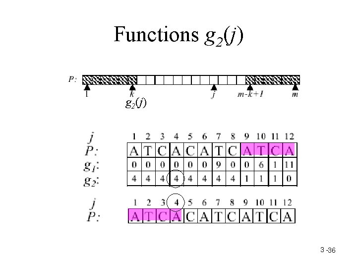
Functions g 2(j) 3 -36

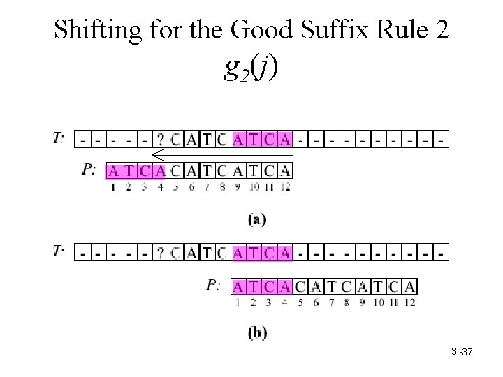
Shifting for the Good Suffix Rule 2 g 2(j) 3 -37

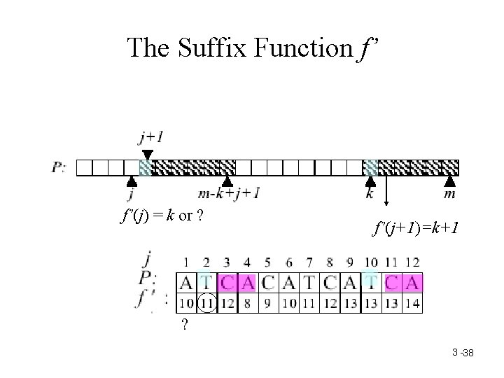
The Suffix Function f’ f’(j) = k or ? f’(j+1)=k+1 ? 3 -38

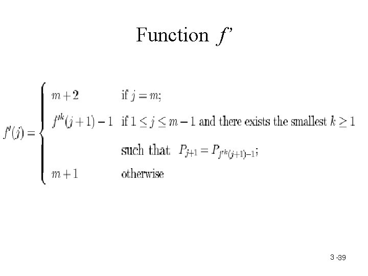
Function f’ 3 -39

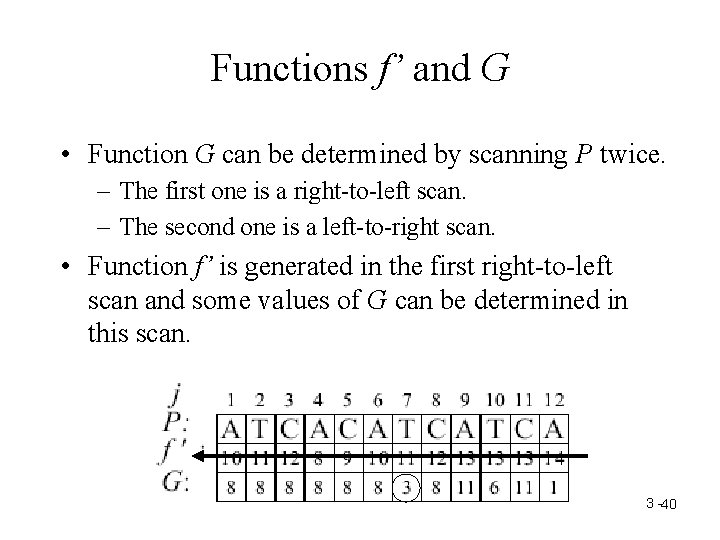
Functions f’ and G • Function G can be determined by scanning P twice. – The first one is a right-to-left scan. – The second one is a left-to-right scan. • Function f’ is generated in the first right-to-left scan and some values of G can be determined in this scan. 3 -40

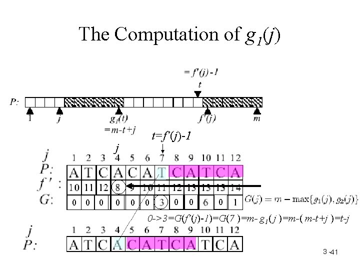
The Computation of g 1(j) t=f’(j)-1 j 0 0 0 0 0 ->3=G(f’(j)-1)=G(7 )=m- g 1( j )=m-( m-t+j )=t-j 3 -41

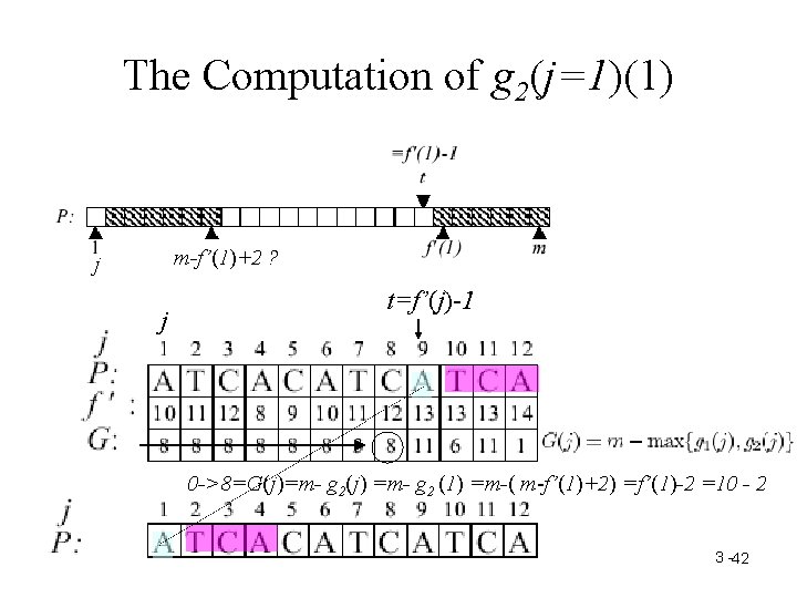
The Computation of g 2(j=1)(1) m-f’(1)+2 ? j j t=f’(j)-1 0 ->8=G(j)=m- g 2(j) =m- g 2 (1) =m-( m-f’(1)+2) =f’(1)-2 =10 - 2 3 -42

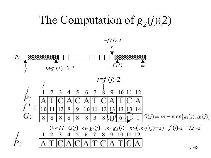
The Computation of g 2(j)(2) m-f’(1)+2 ? j j t=f’(j)-2 0 ->11=G(j)=m- g 2(j) =m- g 2 (j) =m-( m-f’(j)+1) =f’(j)-1 =12 -1 3 -43

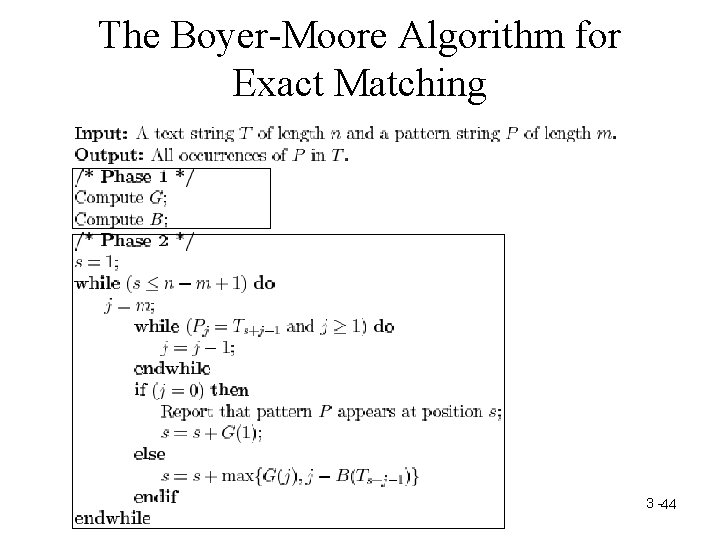
The Boyer-Moore Algorithm for Exact Matching 3 -44

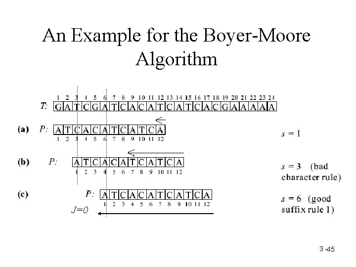
An Example for the Boyer-Moore Algorithm J=0 3 -45

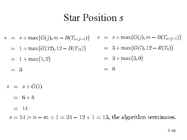
Star Position s 3 -46

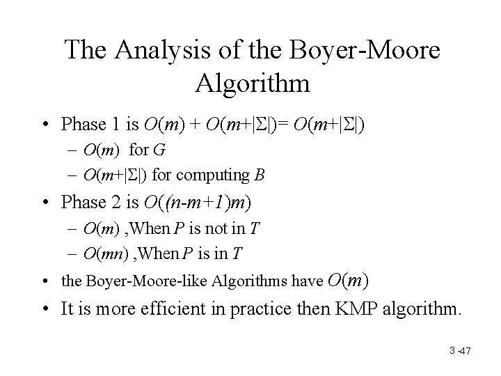
The Analysis of the Boyer-Moore Algorithm • Phase 1 is O(m) + O(m+| |)= O(m+| |) – O(m) for G – O(m+| |) for computing B • Phase 2 is O((n-m+1)m) – O(m) , When P is not in T – O(mn) , When P is in T • the Boyer-Moore-like Algorithms have O(m) • It is more efficient in practice then KMP algorithm. 3 -47

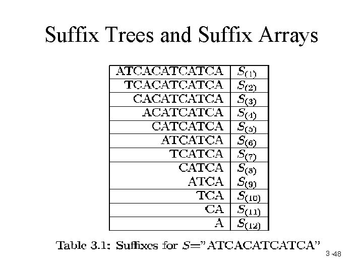
Suffix Trees and Suffix Arrays 3 -48

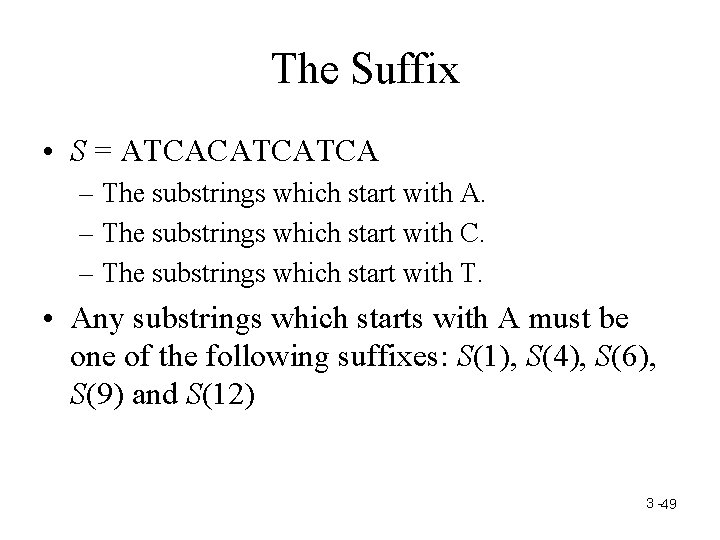
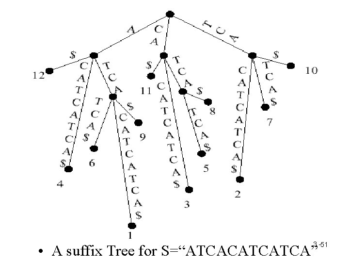
The Suffix • S = ATCACATCATCA – The substrings which start with A. – The substrings which start with C. – The substrings which start with T. • Any substrings which starts with A must be one of the following suffixes: S(1), S(4), S(6), S(9) and S(12) 3 -49

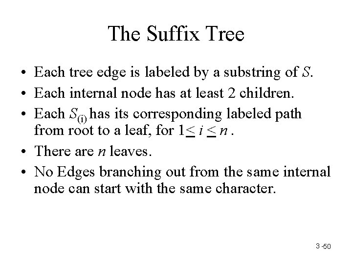
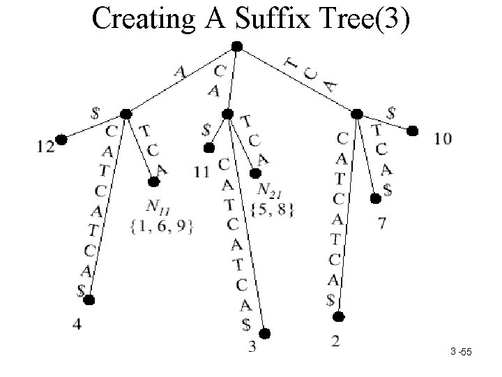
The Suffix Tree • Each tree edge is labeled by a substring of S. • Each internal node has at least 2 children. • Each S(i) has its corresponding labeled path from root to a leaf, for 1< i < n. • There are n leaves. • No Edges branching out from the same internal node can start with the same character. 3 -50

3 -51 • A suffix Tree for S=“ATCACATCATCA”

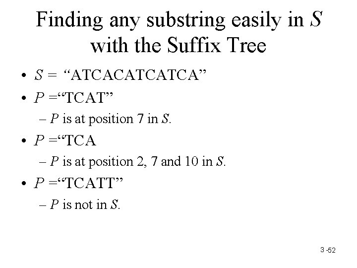
Finding any substring easily in S with the Suffix Tree • S = “ATCACATCATCA” • P =“TCAT” – P is at position 7 in S. • P =“TCA – P is at position 2, 7 and 10 in S. • P =“TCATT” – P is not in S. 3 -52

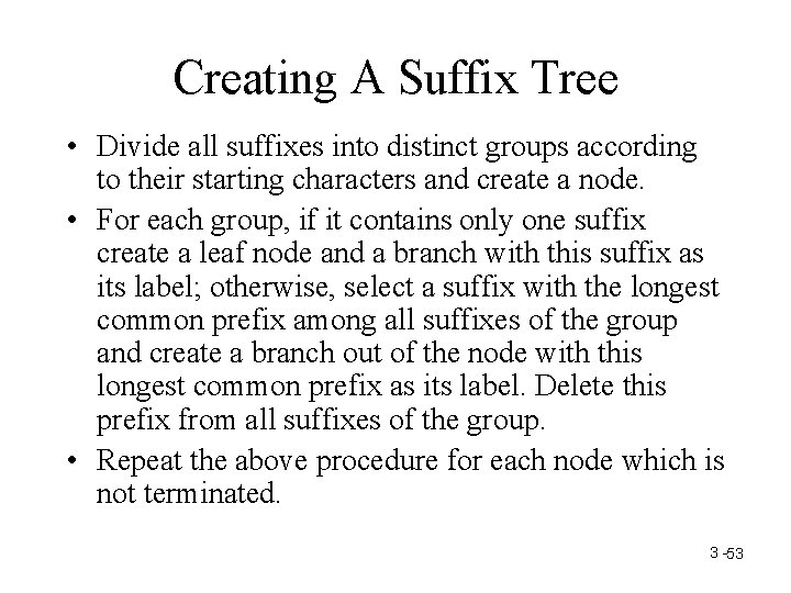
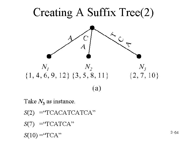
Creating A Suffix Tree • Divide all suffixes into distinct groups according to their starting characters and create a node. • For each group, if it contains only one suffix create a leaf node and a branch with this suffix as its label; otherwise, select a suffix with the longest common prefix among all suffixes of the group and create a branch out of the node with this longest common prefix as its label. Delete this prefix from all suffixes of the group. • Repeat the above procedure for each node which is not terminated. 3 -53

Creating A Suffix Tree(2) Take N 3 as instance. S(2) =“TCACATCATCA” S(7) =“TCATCA” S(10) =“TCA” 3 -54

Creating A Suffix Tree(3) 3 -55

• A suffix tree for a text string T of length n can be constructed in O(n) time. • To search a pattern P of length m on a suffix tree needs O(m) comparisons. • Thus we have an O(n+m) time algorithm for the exact string matching problem. 3 -56

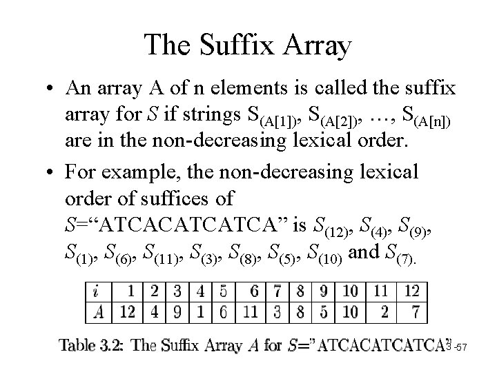
The Suffix Array • An array A of n elements is called the suffix array for S if strings S(A[1]), S(A[2]), …, S(A[n]) are in the non-decreasing lexical order. • For example, the non-decreasing lexical order of suffices of S=“ATCACATCATCA” is S(12), S(4), S(9), S(1), S(6), S(11), S(3), S(8), S(5), S(10) and S(7). 3 -57

• If T is represented by a suffix array, it takes O(mlogn) time to find P in T because a binary search can be conducted on the array. • A suffix array can be determined in O(n) by lexical depth first searching in a suffix tree for a string of length n. • The total time will be O(n+mlogn) time. 3 -58

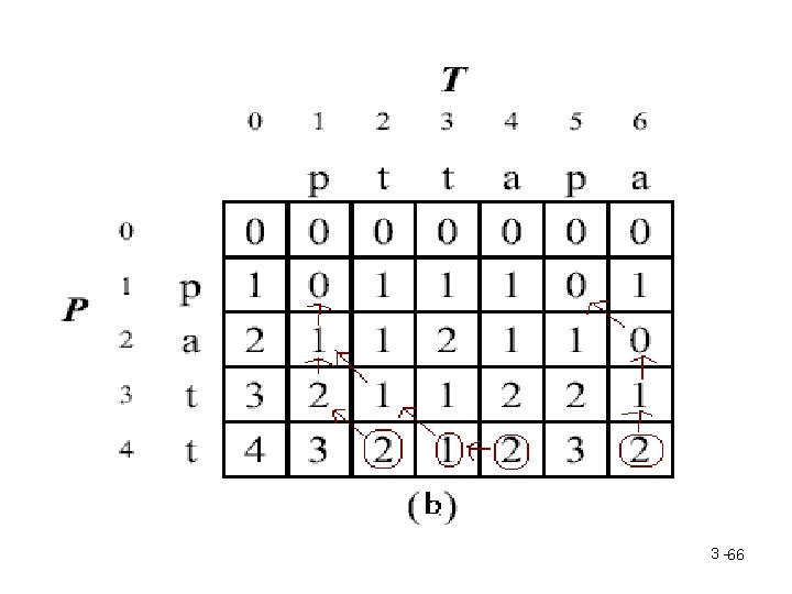
Approximate String Matching • Given a text string T of length n, a pattern string P of length m and a maximal number of errors allowed k, the approximate string matching is to find all text positions where the pattern matches the text up to k errors, where errors can be substituting, deleting, or inserting a character. • For instance, if T =“pttapa’, P =“patt” and k =2, the substrings T 1, 2 , T 1, 3 , T 1, 4 and T 5, 6 are all up to 2 errors with P. 3 -59

The Suffix Edit Distance • Two strings S 1 and S 2. • The suffix edit distance which is the minimum number of substitutions, insertion and deletions, which will transform some suffix of S 1 into S 2. – Consider S 1=“p” and S 2=“p”. The suffix edit distance between S 1 and S 2 is 0. – Consider S 1=“ptt” and S 2=“p”. The suffix edit distance between S 1 and S 2 is 1. 3 -60

• What is the meaning of the suffix edit distance between T and P? • If it is not greater than K, then we know that there is an approximate matching of a suffix of T with P with error not greater than k. That is, we have succeeded in finding a desired approximate matching. 3 -61

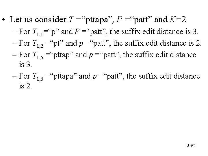
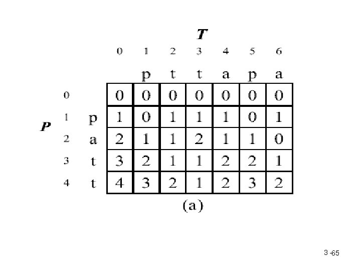
• Let us consider T =“pttapa”, P =“patt” and K=2 – For T 1, 1=“p” and P =“patt”, the suffix edit distance is 3. – For T 1, 2 =“pt” and p =“patt”, the suffix edit distance is 2. – For T 1, 5 =“pttap” and p =“patt”, the suffix edit distance is 3. – For T 1, 6 =“pttapa” and p =“patt”, the suffix edit distance is 2. 3 -62

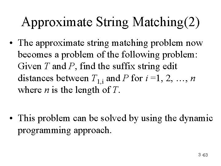
Approximate String Matching(2) • The approximate string matching problem now becomes a problem of the following problem: Given T and P, find the suffix string edit distances between T 1, i and P for i =1, 2, …, n where n is the length of T. • This problem can be solved by using the dynamic programming approach. 3 -63

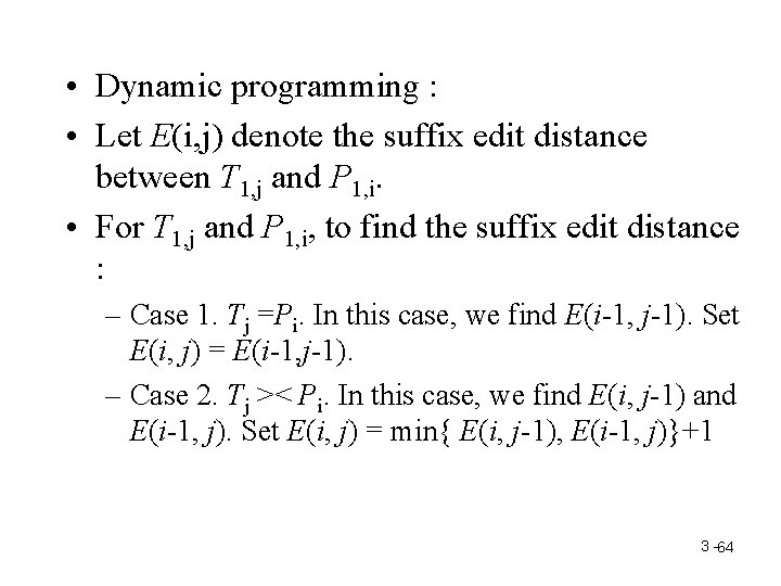
• Dynamic programming : • Let E(i, j) denote the suffix edit distance between T 1, j and P 1, i. • For T 1, j and P 1, i, to find the suffix edit distance : – Case 1. Tj =Pi. In this case, we find E(i-1, j-1). Set E(i, j) = E(i-1, j-1). – Case 2. Tj >< Pi. In this case, we find E(i, j-1) and E(i-1, j). Set E(i, j) = min{ E(i, j-1), E(i-1, j)}+1 3 -64

3 -65

3 -66