Chap 3 Net Present Value Net Present Value

Chap 3 Net Present Value

Net Present Value v v v Net present value is the single most widely used tool for large investments made by corporations. Klammer reported a survey of over 100 large companies indicating that in 1959 only 19 percent used NPV techniques, but by 1970, 57 percent used them. Roughly a decade later, Schall, Sundem, and Geijsbeek sampled 424 large firms and found that 86 percent of those responding used NPV. It took over two decades for NPV to be widely accepted. Undoubtedly, this rate of adoption was affected by the introduction of pocket calculators and desktop personal computers.

Net Present Value v v We want to review NPV carefully because it is the foundation for real options analysis. ” The separation principle ” : it shows that the shareholders of a firm will, regardless of their individual rates of time preference, unanimously agree that the managers of the firm should maximize shareholders’ wealth by taking investments that earn at least the market-determined opportunity cost of capital. Free cash flows of the project, the weighted average cost of capital, The equivalence of the risk-adjusted and the certainty-equivalent methods of estimating the NPV of a project.

The separation principle v v v Simple stated, the separation principle is the useful result that shareholders of a firm will agree about the decision rule they want managers to execute on their behalf – namely to undertake investments until the marginal return on the last dollar invested is greater than or equal to the market-determined opportunity cost of capital. Shareholders do not have to take a vote – they will unanimously agree. This is a critical keystone in theory of decision making because we do not have to construct a complicated rule for the managers that requires that they acquire and use individual owner ( shareholder ) preferences.

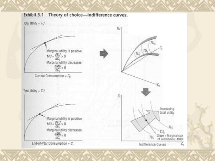
Shows the rate of exchange between consumption today and consumption at the end of the year that will leave Mr. Crusoe with the same total utility. v In effect, his marginal rate of substitution is his subjective price of units of consumption tomorrow for units of consumption today. v He always requires extra units of consumption tomorrow in return for giving up a unit of consumption today. v

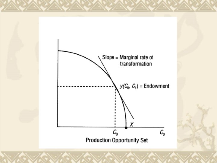
v The slope of a line drawn tangent to it is called the marginal rate of transformation.

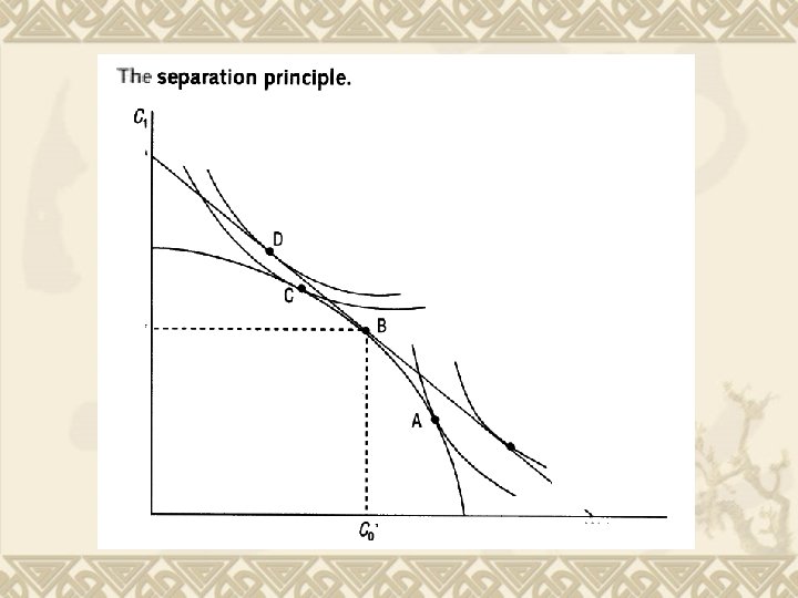
v Marginal rate of substitution equals his marginal rate of transformation. v He will decide to remain at point B, where he consumes today and at the end of the period, and invests today. v Won’t they all choose different optimal consumption/production points because they all have different preferences for consumption over time, and therefore difference indifference curves? The answer is no.

Note that the production output at point B, which is where the market line is just tangent to the production opportunity set, provides him with the greatest feasible wealth, . v It also provides him with the highest possible total utility, because he will produce the output at point B, then borrow against it at rate r to reach point C, a bundle of consumption with wealth. v

v At point C, his marginal rate of substitution is the slope of the market line [ i. e. , - (1 + r)]. v Also, the same market line is tangent to the production opportunity set at point B. v Therefore, if he maximizes his wealth, and his total utility, he will choose to produce the combination at point B, then borrow to move to point C. v At point C, his marginal rate of substitution equals the slope of the market line, which in turn equals his marginal rate of transformation.

v Therefore, all individuals, regardless of their time preferences for consumption today versus consumption tomorrow, will choose to invest until the marginal rate of return on the last unit of investment is just equal to the market rate ( at point B ). v This separation principle means that the wealthmaximizing rule for investment is separate from any information about individual utility functions.

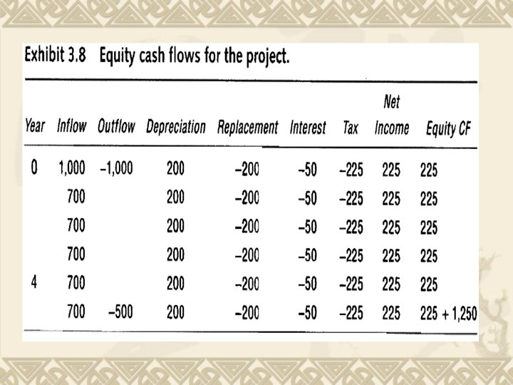
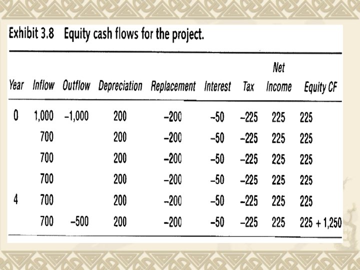
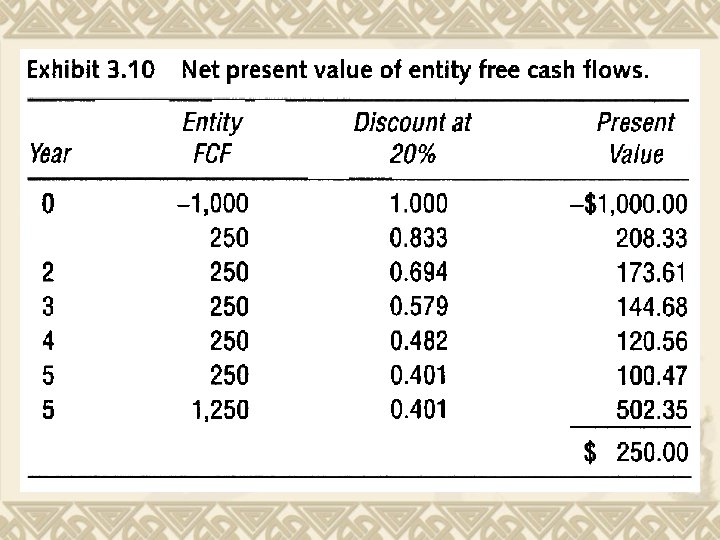
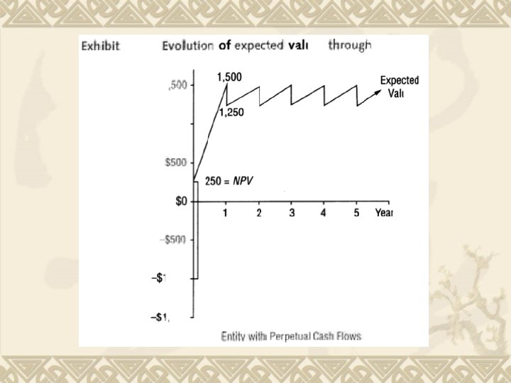
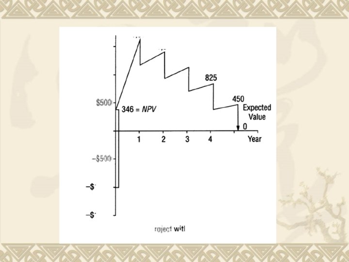
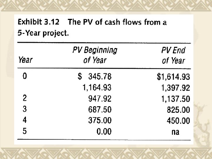
Estimating free cash flows v The first step will always be to estimate the present value of the project without flexibility. v The free cash flows that are payable to both sources of capital – debt and equity.

v Adding these values together gives the value of the firm, $1, 250. v The shareholders receive $1, 250 in year 5 but must pay $500 to bondholders.

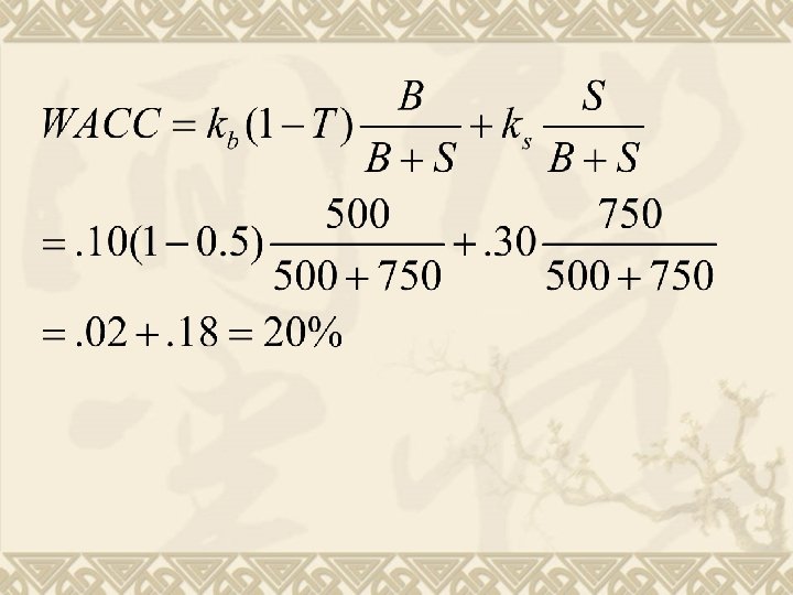
The weighted average cost of capital ( WACC ) The weighted average cost of capital is the weighted average of the after-tax marginal costs of capital. v It is appropriate for discounting entity or project cash flows because these cash flows are available for payment to both sources of capital – debt and equity. v Market value weights are used because the market value of capital committed, not the book value, determines the cash flow required on investment. v

v We find other debt with the same risk and assume that its yield to maturity is the same as ours. v Comparable securities in the capital markets to estimate the capital for our project.

v One of the advantages of discounting the firm’s free cash flows at the after-tax weight average cost of capital is that this technique separates the investment decisions of the firm from its financing decisions. v The definition of free cash flows shows what the firm will earn after taxes assuming that it has no debt capital.

v Thus, changes in the assumed debt-to-equity ratio have no effect on the definition of cash flows for capital budgeting purposes. v The effect of financial decisions is reflected in the cost of capital.

Certainty-equivalent approach to net present value It is possible to estimate the value of a project either by taking its expected future free cash flows and discounting them at a risk-adjusted weighted average cost of capital, or to risk-adjust the cash flows and discount them at the risk-free rate. v The answer should be the same either way. v The certainty-equivalent approach is a common method for valuing options in a lattice. v

v Consider a simple one-period example. v A project’s expected cash flows are $1, 000, the risk-free rate is 10 percent, the expected rate of return on the market is 17 percent, and the project’s beta is 1. 5. v If it is an all-equity firm, then its present value is

v If the investment outlay is $800, then its net present value is NPV = PV – I = $829. 88 - $800 = $29. 88

is the market price of risk in the capital asset pricing model. v This approach adjusts for risk by subtracting a penalty from expected cash flows to first obtain certainty-equivalent cash flows, then it discounts them at the risk-free rate. v $1, 000 - $87. 13 = $912. 87 v

v That we can obtain the same answer using either a risk-adjusted or a risk-neutral approach.

Differences between the net present value and the real options approaches v Note that the uncertainty of cash flows is not explicitly modeled in the NPV approach. v One merely discounts expected cash flows.

v The problem solution is to compare all possible mutually exclusive routes to determine their value, , then to choose the best among them.

v Mathematically, a call option is an expectation of maximums ( not a maximum of expectations ) :