Chap 2 Basics of hydraulics Advantages of hydraulic

Chap 2 Basics of hydraulics Advantages of hydraulic control： ― easy of control ― high power output ― good dynamic response ― good dissipation of heat Disadvantages： ― high energy losses ― possibility of leakages（dirty） § Work w = F×L where w：work（N˙m） F：Force（N） L：Distance（m） § Pascal´s Law（Multiplication of force） p = = = constant w = F 1 L 1 = F 2 L 2 （assume no energy losses）

Power P= = = F × =（p × A）（ ）= p × Q where P：power p：pressure Q：flow rate （ ） F 1 L 1 F 2 L 2 A 1 A 2

P= （k. W） 1 W = Ex：How to derive？ HP（horsepower）= In the case of rotary actuator（motor） Q n 1 V 1 Pn n 2 V 2 T 1 T 2 For pump： V 1=A×πd Q 1=n 1×V 1 Where Q: Flow rate V 1: Displacement of pump T: Torque

For motor： Piston V 2 = A ×πd Q 2 = n 2 × V 2 If Q 1= Q 2 n 1 v 1=n 2 v 2 = A

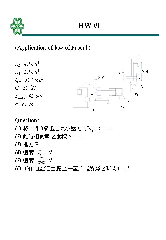
HW #2 Q Given : n 1 =1450 rpm n 2 =400 rpm T 2=250 N-m Pn=200 bar V 1 n 1 T 1 Pn V 2 n 2 T 2 Please calculate: (1) The optimal displacement of motor V 2 = ? Note: as follows are different types to choose : V 2 = 40 / 56 / 71 / 90 / 125 cm 3/rev (2) Pressure Pn= ? , Flow rate Q= ? , Displacement of pump V 1= ? and the Power P = ? (according to the chosen V 2)

Torque T 1= F × di =（A×ΔP） =（ ）×Δp× = = similarly： T 2 = Torque transfer relation： = Assume no energy loss： P 1= T 1 w 1 = × 2π× n 1 =V 1× n 1 ×Δp =Q 1 ×Δp Output power of motor： P 2=Q 2×Δp Total efficiency=η= =1（ideal case）

Conservation of Mass（Continuity Equation） + =0 ρ1 A 1 V 1 ρ2 A 2 V 2 =ρ1 Q 1=ρ1 A 1 V 1 =ρ2 Q 2=ρ2 A 2 V 2 pipe if ρ1=ρ2 （incompressible fluid） then V 1 A 1=V 2 A 2 Ex： A V 1 A 1ρV 1－A 2ρV 2－Aρ =0 If ρ: constant V 1 A 1 －V 2 A 2 = A V 2 A 2

Conservation of Energy（Bernoulli’s Equation） P 2 V 2 P 1 V 1 h 1 1 h 2 2

Total Energy at any point = Elevation＋Pressure＋Kinetic = mgh＋ ＋ Bernoulli’s equation： ＋ ＋h 1= ＋ ＋h 2 Ex 1：（continuity equation） Q=25 A 1 A 2 D=50 mm d d=30 mm D d 1=d 2=15 mm d 2 d 1 Q

Questions： Piston velocity =？ Velocities of the fluid in the inlet and outlet pipes = ? Answer： （1） A 1= πD 2=19. 6㎝ 2 A 2= π(D 2－d 2）=12. 56㎝ 2 Cross section area of inlet and outlet pipes A 3= πd 12=1. 77㎝ 2 Piston velocity V 1= =0. 21 （2）Velocity of the fluid in inlet pipe： V 3= =2. 36 From continuity equation： Where V 4 ：velocity of the fluid in outlet pipe Thus V 4= =1. 49

Ex 2（Application of Bernoulli’s equation） ρ=0. 8 =800 P 1 70 bar P 2 d 2=0. 5 cm d 1=3 cm V 1 V 2 Q=10 l/min Assume：no work and no energy dissipation Question：P 2=？ Answer： h 1=h 2 ； ρ1=ρ2 V 1= = V 2=（ = 0. 236 ）2×V 1= 8. 496 From Bernoulli’s equation： + = + P 2=69. 7× 105 =69. 7 bar (Pressure drop ： 0. 3 bar)

Flow through orifice ∵ A 2 «A 1 ∴V 1 «V 2 P 1+ 1/2 ρV 12 = P 2 + 1/2 ρV 22 where Δp＊=P 1－P 2 V 2= Flow rate Q=A 2×V 2 =A 2× 1 0 2 3

Area A 2=Cc×A 0 Where Cc：contraction coefficient Flow coefficient Cf Q = Cf × A 0 × where Δp=P 1－P 3 Cf = f（Reynolds number；geometry） =0. 6~1. 0 Valve geometry P 0 Q = Cf ×πd × d P 1 Q C f = 0. 6~0. 64

Theory of Momentum (Principle of impulse) = m （momentum） = = = +m F A 1 F 1 Q F 2 F 1 CV F 2 2 Q F 1 A 2 (Vector)

Steady flow （ = 0） position 1： =ρ1 Q 1 = ρ1 Q 1 position 2： =ρ2 Q 2 = - ρ2 Q 2 Flow force： = + = - - Ex: assume incompressible （ρ=const） ρ1 Q 1=ρ2 Q 2 = ρQ = -ρQ（ + ） unsteady part ： m CV

Assume incompressible = const Thus Q 1= Q 2 = Q = - = （A：const） = ×m（∵ = - ∴steady part=0） =ρ A × pressure drop：P 1 -P 2 = = × （Q = v‧A） F =A（P 1 -P 2） Where ：hydraulic inductance

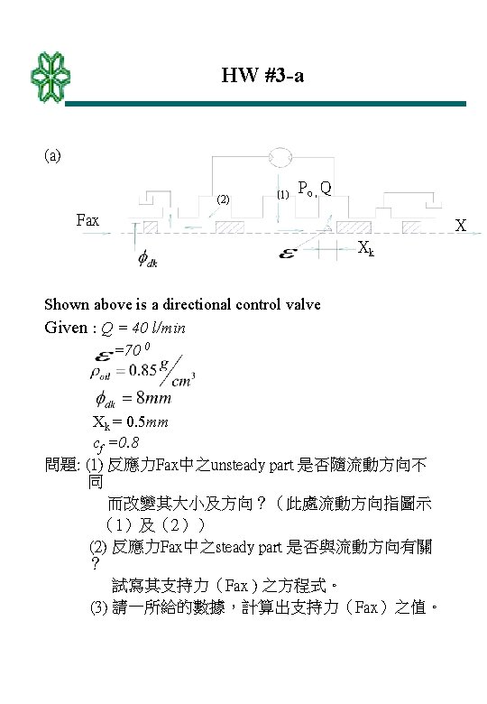
Flow force on the directional control valve （a） Recall Fstr= F 1 - F 2 = Fi - Fo (scalar) Fax= -Fstr = Fo- Fi Fax= cosε 0 - cosεi - ρ Io εi ε 2 εo ε 1 Ii Io Ii Fax Fstr 2 1

= ρv 2 × Q = ρv 1 × Q εo= ε 2= 90 o εi= ε 1 + 180 o Fax=0 + ρv 1 Qcosε 1 - ρ εi （b） ε 2 Fax= Io Ii cosε 0 - εo, ε 1 cosεi + ρ =ρv 1 Q ε 0=ε 1 =ρv 2 Q εE=ε 2+1800=2700 Fax=ρv 1 Qcosε 1+ ρ

HW#3 -b （b ) Laminar flow through eccentric clearance P 1 P 2 D d d=2 cm , l= 1 cm , =50 cst , Questions : (1) Qe=0 = ? ( l / min) (2) Qe= = ? ( l / min) =0. 85 , e

Case 1：small orifice area （ ~const） Q= Cf × A × v= = Cf × Where A=orifice area =πd x x d

by small orifice area Δp~const Fstr thus Q ~ X Fstr=ρv cosε （only steady part） =ρv（v. A）cosε =2 Cf 2 ×πd x ×Δpcosε Cs×X Case 2：large orifice area （Q~const） Fstr= cosε Fstr Thus Fstr~ Fstr x Pmax Q linear Pmax=const Q Q 1 Q 2 3 x Small A Large A Q 3>Q 2>Q 1 P 3 max P 2 max P 1 max P 3 max>P 2 max > P 3 max x

Viscosity of fluid U F h Shear stress where : dynamic viscosity cf. : kinematic viscosity Unit : 1 Poise=1 =0. 1

1 cp=10 -2 Poise =10 -3 1 stoke =1 1 cst=1 η（or ν）= f（T，P） Flow in Pipes Eqs. derived from viscous flow condition （1）laminar flow NR＜ 2000 （2）turbulent flow NR＞ 4000 only empirical Eqs. Reynolds number NR（dimensionless） NR = where V：velocity of fluid DH：hydraulic diameter ν：kinematic viscosity Hydraulic Diameter DH = where A：Area of pipe U：circumference of pipe For pipes： DH= （diameter of pipe）

For narrow clearance h Q b DH= (if h << b) Conclusion: Design in hydraulics Laminar flow

§ Hagen-Poiseuille formula V r y P 1 P 2 （laminar flow in a pipe） =（P 1 -P 2）πy 2 τ× 2πy τ=η = × = v= （r 2 -y 2） for y =0 then Q= = = （P 1 -P 2） Vmax

Laminar flow through the clearance y V h Q Vmax V= （h 2 -4 y 2） Vmax= h 2 Q =2 =2 Q= （P 1 -P 2） b

Laminar flow through eccentric clearance P 1 P 2 Q Q= D e d （P 1 -P 2） Where η：dynamic viscosity （e. g. Poise； When e=Δr, which implies max. eccentricity Q e= 2. 5 Qe=0 ）

Flow through resistance and orifice (a) Resistance 2 r P 1 Q= P 2 Δp =k 1 Δp Q~Δp ~ (b) Orifice P 1 P 2

Q=Cf. A =k 2 Q~ Thus Q orifice Resistance Δp

Pressure losses through pipes Darcy-Weisbach formula： Pf = λ（ ） or hf =λ（ ） where Pf：pressure loss hf ：head loss ：length of pipe d ：internal diameter of pipe λ ：friction factor（derived experimentally）

Example：Laminar pipe flow Q= Δp Q=A×v=πr 2 v Thus Δp =P 1 -P 2 = Pf = λ= = v λ （valid only if Re＜ 2000） For turbulent flow： Blasius formula： λ= （for pipes with smooth inside surface） （3000＜Re＜ 105）

k-values for fluid through sudden expansion, contraction, pipe fitting, valves and bends ΔPff = k × （for turbulent flow） or hff = k（ ） where ΔPff：pressure loss hff：head loss Sudden enlargement: k =（1 - ）2 Q D 1 D 2 Sudden reduction: D 2 Q k = 0. 5（1 - ） D 1 k-values for pipe fitting, valves, and bends are determined empirically

Circuit Calculation k 1 d 1 k 3 1 k 2 2 （P 1+ = +ρgζ 1）-（P 2+ + +ρgζ 2）=ΔPf

HW#4 -a

HW#4 -b

EX: 泵油之空穴(Cavitation of oil pump) A B P 1 ：泵之入口壓力 P 2 ：泵內之最低壓力 Pa ：大氣壓力 Pg ：空氣分離壓力 Pa P 1 P 2 (1) From Bernoulli’s Eq. he (head loss) (2) (3) Define (Net Positive Suction Head) (4) No cavitation (A)