Chap 11 Introduction to Jump Process Stochastic Calculus

Chap 11. Introduction to Jump Process Stochastic Calculus for Finance II Steven E. Shreve 財研二 范育誠

AGENDA � 11. 5 Stochastic Calculus for Jump Process � 11. 5. 1 Ito-Doeblin Formula for One Jump Process � 11. 5. 2 Ito-Doeblin Formula for Multiple Jump Process � 11. 6 Change of Measure � 11. 7 Pricing a European Call in Jump Model

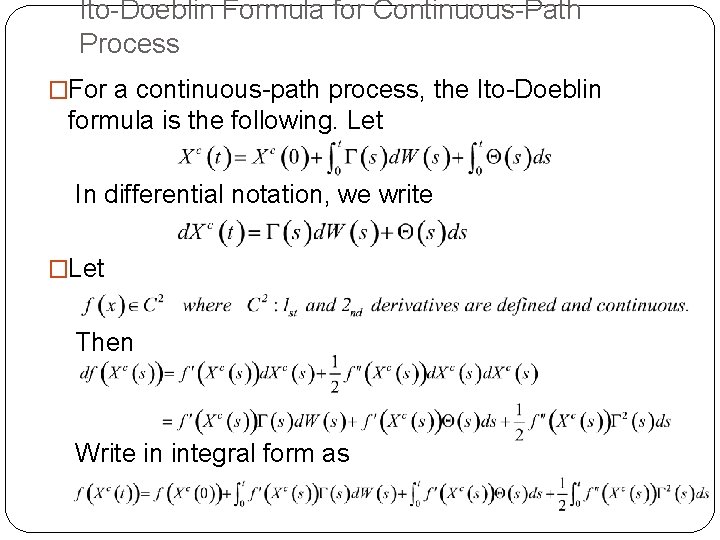
Ito-Doeblin Formula for Continuous-Path Process �For a continuous-path process, the Ito-Doeblin formula is the following. Let In differential notation, we write �Let Then Write in integral form as

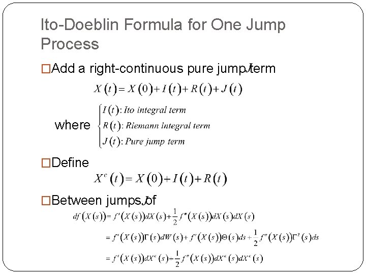
Ito-Doeblin Formula for One Jump Process �Add a right-continuous pure jump term where �Define �Between jumps of

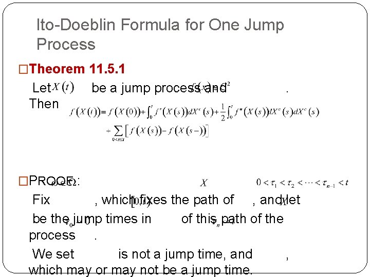
Ito-Doeblin Formula for One Jump Process �Theorem 11. 5. 1 Let Then be a jump process and . �PROOF : Fix , which fixes the path of , and let be the jump times in of this path of the process. We set is not a jump time, and , which may or may not be a jump time.

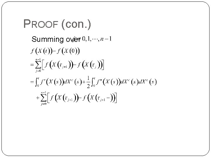
PROOF (con. ) Whenever , Letting continuity of We conclude that Now add the jump in and using the right- at time

PROOF (con. ) Summing over

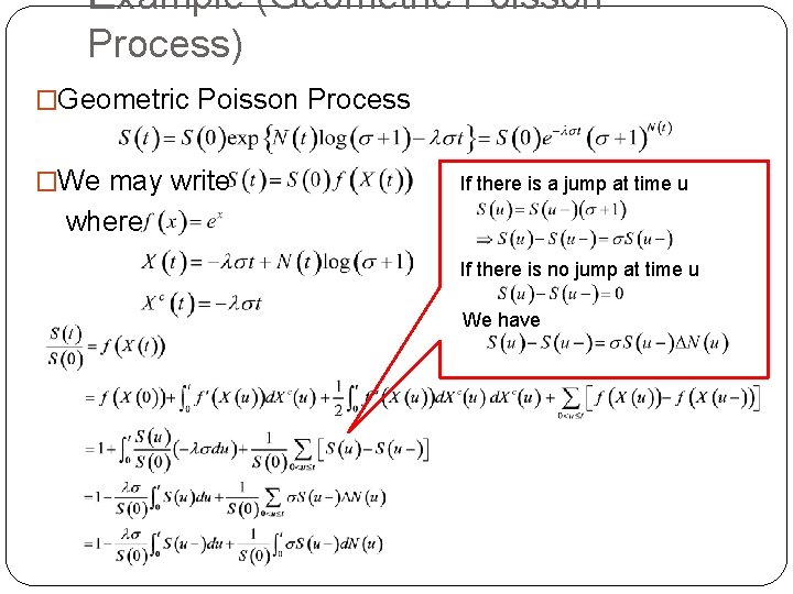
Example (Geometric Poisson Process) �Geometric Poisson Process �We may write If there is a jump at time u where If there is no jump at time u We have

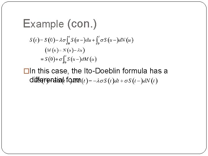
Example (con. ) �In this case, the Ito-Doeblin formula has a differential form

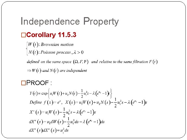
Independence Property �Corollary 11. 5. 3 �PROOF :

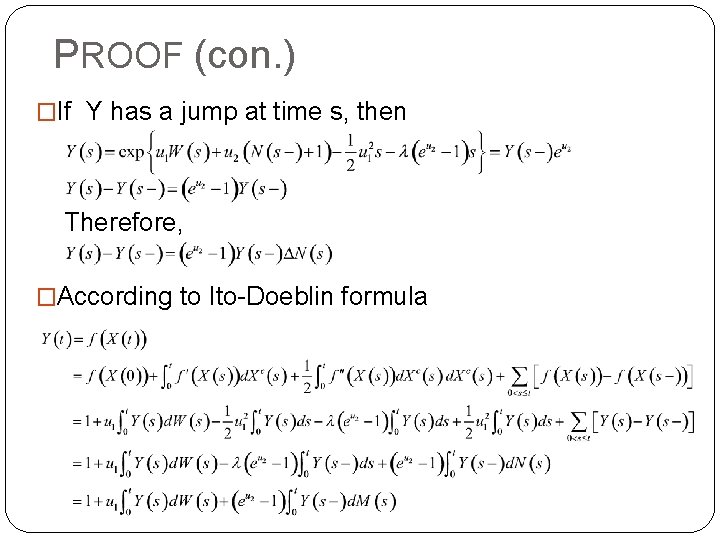
PROOF (con. ) �If Y has a jump at time s, then Therefore, �According to Ito-Doeblin formula

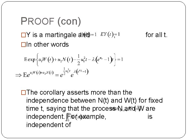
PROOF (con) �Y is a martingale and , for all t. �In other words �The corollary asserts more than the independence between N(t) and W(t) for fixed time t, saying that the process N and W are independent. For example, is independent of

AGENDA � 11. 5 Stochastic Calculus for Jump Process � 11. 5. 1 Ito-Doeblin Formula for One Jump Process � 11. 5. 2 Ito-Doeblin Formula for Multiple Jump Process � 11. 6 Change of Measure � 11. 7 Pricing a European Call in Jump Model

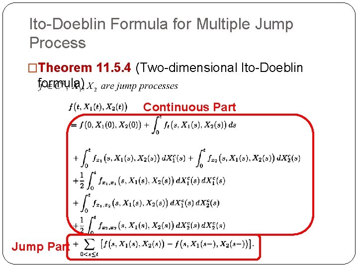
Ito-Doeblin Formula for Multiple Jump Process �Theorem 11. 5. 4 (Two-dimensional Ito-Doeblin formula) Continuous Part Jump Part

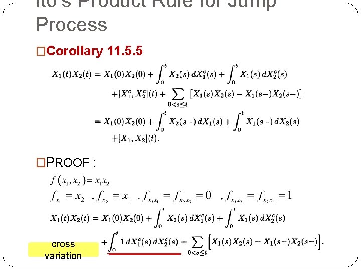
Ito’s Product Rule for Jump Process �Corollary 11. 5. 5 �PROOF : cross variation

PROOF (con. ) � jump parts of , and are pure , respectively.

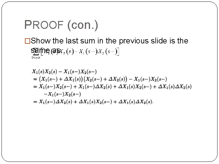
PROOF (con. ) �Show the last sum in the previous slide is the same as

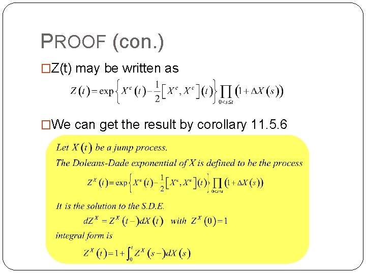
Doleans-Dade Exponential �Corollary 11. 5. 6

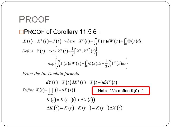
PROOF �PROOF of Corollary 11. 5. 6 : Note : We define K(0)=1

PROOF (con. ) �Use Ito’s product rule for jump process to obtain [Y, K](t)=0

AGENDA � 11. 5 Stochastic Calculus for Jump Process � 11. 6 Change of Measure � 11. 6. 1 Change of Measure for a Poisson Process � 11. 6. 2 Change of Measure for a Compound Poisson Process � 11. 6. 3 Change of Measure for a Compound Poisson Process and a Brownian Motion � 11. 7 Pricing a European Call in Jump Model

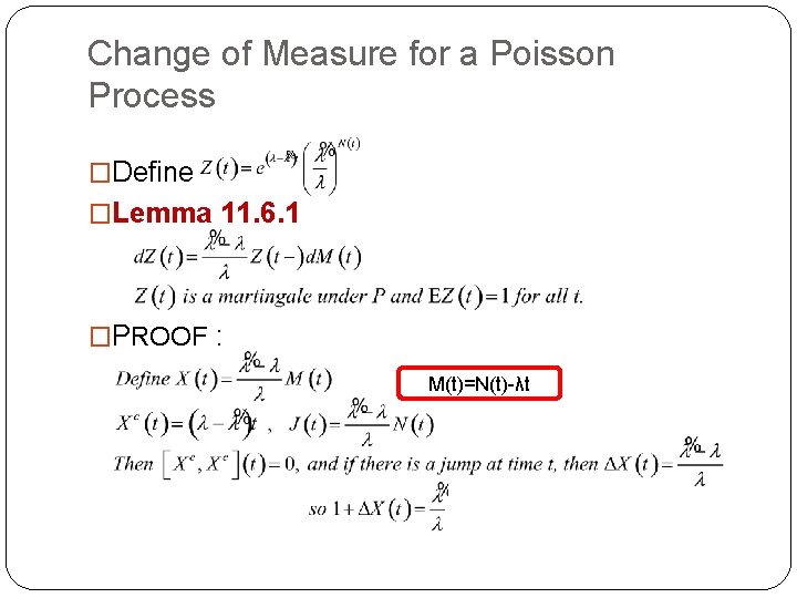
Change of Measure for a Poisson Process �Define �Lemma 11. 6. 1 �PROOF : M(t)=N(t)-λt

PROOF (con. ) �Z(t) may be written as �We can get the result by corollary 11. 5. 6

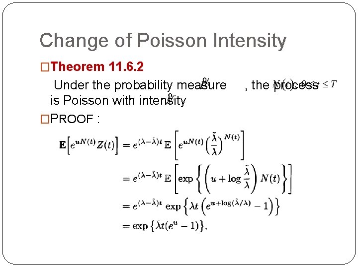
Change of Poisson Intensity �Theorem 11. 6. 2 Under the probability measure is Poisson with intensity �PROOF : , the process

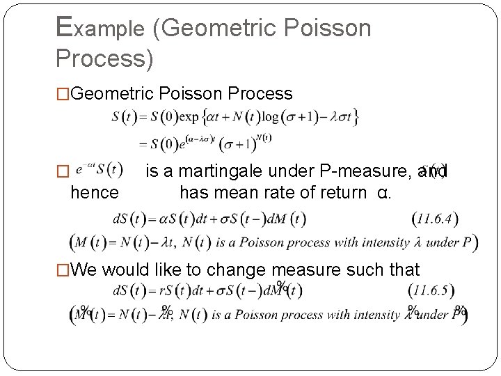
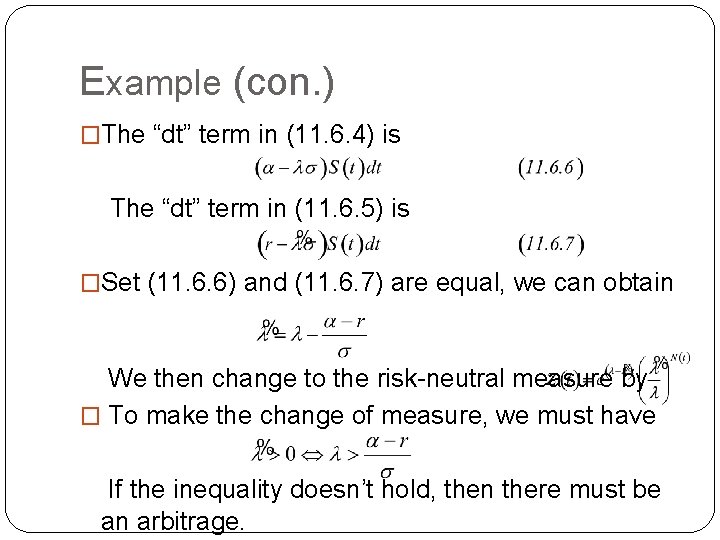
Example (Geometric Poisson Process) �Geometric Poisson Process � hence is a martingale under P-measure, and has mean rate of return α. �We would like to change measure such that

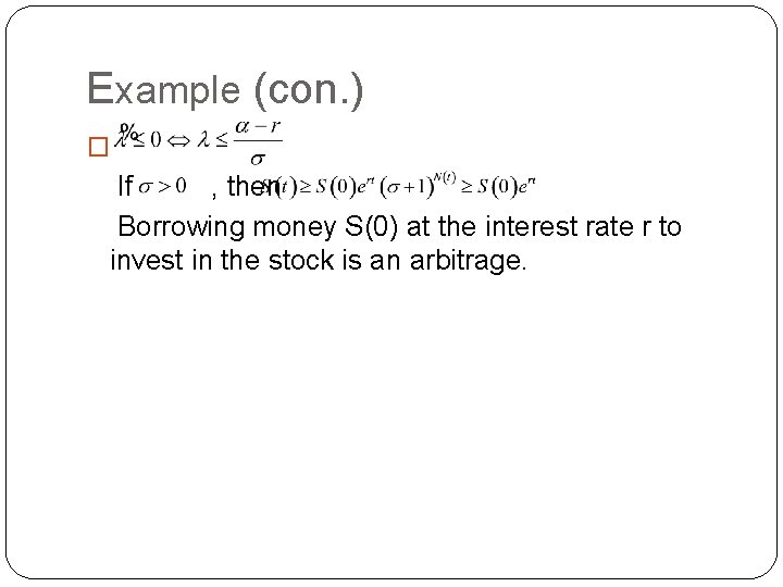
Example (con. ) �The “dt” term in (11. 6. 4) is The “dt” term in (11. 6. 5) is �Set (11. 6. 6) and (11. 6. 7) are equal, we can obtain We then change to the risk-neutral measure by � To make the change of measure, we must have If the inequality doesn’t hold, then there must be an arbitrage.

Example (con. ) � If , then Borrowing money S(0) at the interest rate r to invest in the stock is an arbitrage.

AGENDA � 11. 5 Stochastic Calculus for Jump Process � 11. 6 Change of Measure � 11. 6. 1 Change of Measure for a Poisson Process � 11. 6. 2 Change of Measure for a Compound Poisson Process � 11. 6. 3 Change of Measure for a Compound Poisson Process and a Brownian Motion � 11. 7 Pricing a European Call in Jump Model

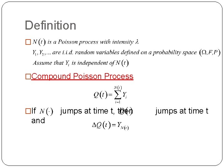
Definition � �Compound Poisson Process �If and jumps at time t, then jumps at time t

Jump-Size R. V. have a Discrete Distribution takes one of finitely many possible nonzero values � �According to Corollary 11. 3. 4

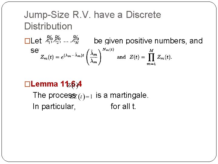
Jump-Size R. V. have a Discrete Distribution �Let be given positive numbers, and set �Lemma 11. 6. 4 The process In particular, is a martingale. for all t.

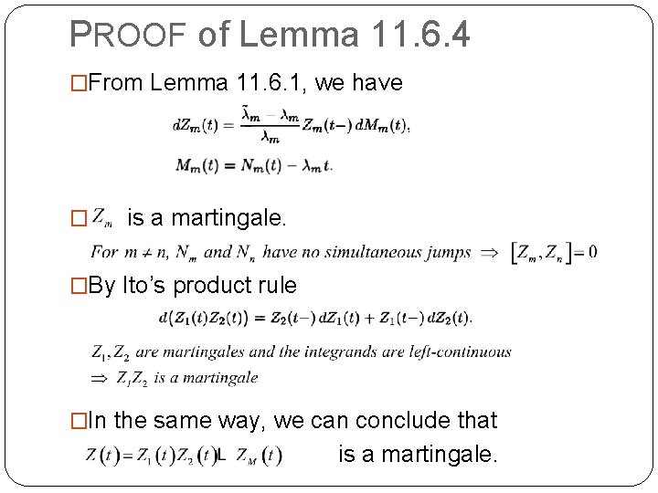
PROOF of Lemma 11. 6. 4 �From Lemma 11. 6. 1, we have � is a martingale. �By Ito’s product rule �In the same way, we can conclude that is a martingale.

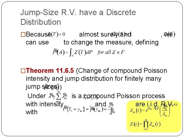
Jump-Size R. V. have a Discrete Distribution �Because can use almost surely and , we to change the measure, defining �Theorem 11. 6. 5 (Change of compound Poisson intensity and jump distribution for finitely many jump sizes) Under , is a compound Poisson process with intensity , and are i. i. d. R. V. with

PROOF of Theorem 11. 6. 5

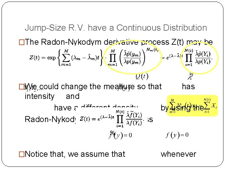
Jump-Size R. V. have a Continuous Distribution �The Radon-Nykodym derivative process Z(t) may be written as �We could change the measure so that has intensity and have a different density by using the Radon-Nykodym derivative process �Notice that, we assume that whenever

AGENDA � 11. 5 Stochastic Calculus for Jump Process � 11. 6 Change of Measure � 11. 6. 1 Change of Measure for a Poisson Process � 11. 6. 2 Change of Measure for a Compound Poisson Process � 11. 6. 3 Change of Measure for a Compound Poisson Process and a Brownian Motion � 11. 7 Pricing a European Call in Jump Model

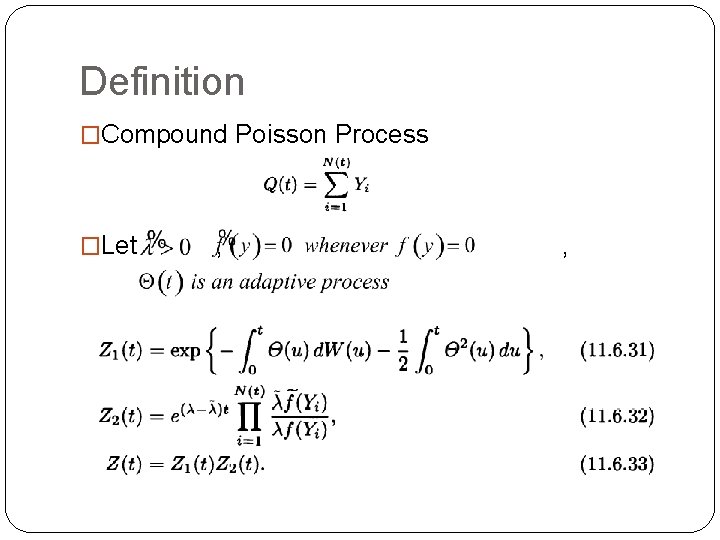
Definition �Compound Poisson Process �Let , ,

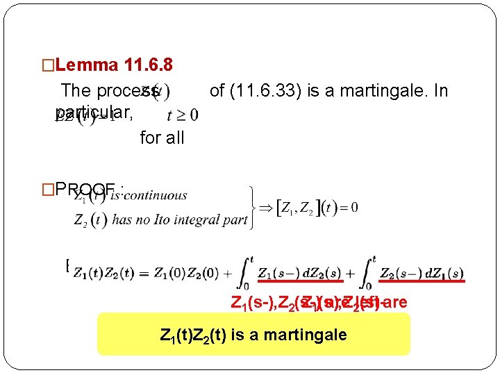
�Lemma 11. 6. 8 The process particular, for all of (11. 6. 33) is a martingale. In �PROOF : By Ito’s product rule, Z 1(s-), Z 2(s-) are 2 left. Z 1(s), Z (s) are continuous martingales Z 1(t)Z 2(t) is a martingale

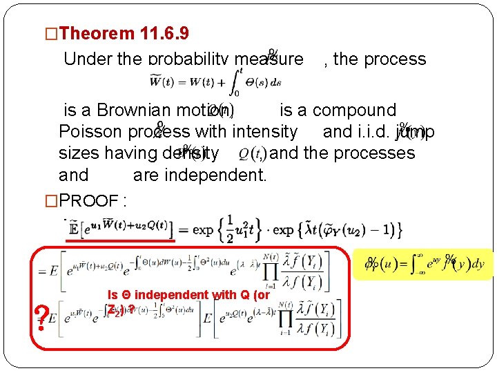
�Theorem 11. 6. 9 Under the probability measure , the process is a Brownian motion, is a compound Poisson process with intensity and i. i. d. jump sizes having density , and the processes and are independent. �PROOF : The key step in the proof is to show ？ Is Θ independent with Q (or Z 2 ) ?

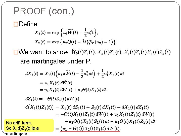
PROOF (con. ) �Define �We want to show that are martingales under P. No drift term. So X 1(t)Z 1(t) is a martingale

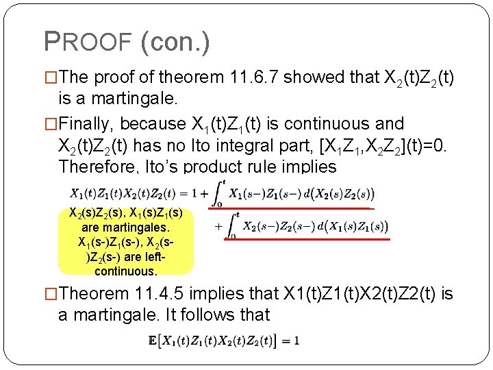
PROOF (con. ) �The proof of theorem 11. 6. 7 showed that X 2(t)Z 2(t) is a martingale. �Finally, because X 1(t)Z 1(t) is continuous and X 2(t)Z 2(t) has no Ito integral part, [X 1 Z 1, X 2 Z 2](t)=0. Therefore, Ito’s product rule implies X 2(s)Z 2(s), X 1(s)Z 1(s) are martingales. X 1(s-)Z 1(s-), X 2(s)Z 2(s-) are leftcontinuous. �Theorem 11. 4. 5 implies that X 1(t)Z 1(t)X 2(t)Z 2(t) is a martingale. It follows that

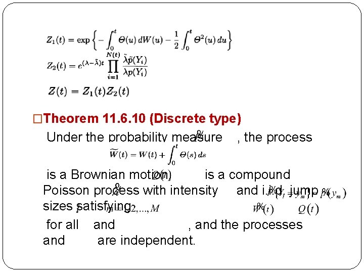
�Theorem 11. 6. 10 (Discrete type) Under the probability measure , the process is a Brownian motion, is a compound Poisson process with intensity and i. i. d. jump sizes satisfying for all and , and the processes and are independent.

AGENDA � 11. 5 Stochastic Calculus for Jump Process � 11. 6 Change of Measure � 11. 7 Pricing a European Call in Jump Model � 11. 7. 2 Asset Driven by Brownian Motion and Compound Poisson Process

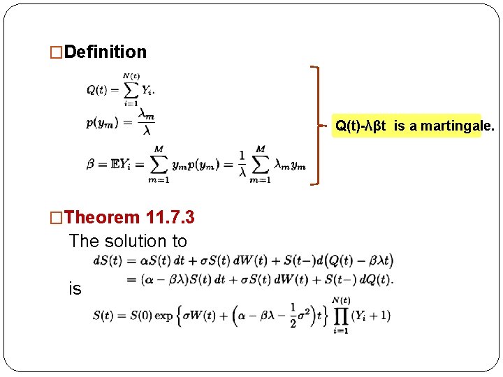
�Definition Q(t)-λβt is a martingale. �Theorem 11. 7. 3 The solution to is

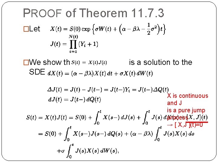
PROOF of Theorem 11. 7. 3 �Let �We show that is a solution to the SDE. X is continuous and J is a pure jump process → [ X, J ](t)=0

PROOF (con. ) �The equation in differential form is